1 Tariffs and Quotas with Home Monopoly
1. No-Trade Equilibrium
Standard monopoly model with increasing MC: Produce where P > MC = MR.
a. Comparison with Perfect Competition: In a competitive market P=MC; the monopolist restricts its quantity in order to raise price relative to the competitive equilibrium.
2. Free-Trade Equilibrium
Trade makes the monopolist’s demand curve perfectly elastic at the world price. It produces where the world price = MC. Home consumers demand more than the amount supplied by the monopolist, so the country imports the good.
a. Comparison with Perfect Competition
Monopolist acts exactly as a competitive industry would in a small open economy. Free trade also creates gains from trade by reducing monopoly power.
3. Effect of a Home Tariff
The monopolist’s demand curve shifts up vertically by the amount of the tariff. It increases production, while consumers reduce quantity demanded. Therefore imports decrease.
a. Comparison with Perfect Competition
The effects of the tariff are exactly the same as they would be in a competitive market.
b. Home Loss Due to the Tariff
Exactly the same as in Chapter 8
4. Effect of a Home Quota
The quota shelters the monopoly from foreign competition, so prices increase more, and the deadweight loss is greater, than for a tariff. The quota shifts back effective demand of the monopolist. Price is higher and quantity lower than with tariff.
a. Home Loss Due to the Quota
Tariff versus quota: Greater loss to consumers by the quota, but greater profit. The calculation of the deadweight loss for the quota is complicated, but it is always greater than for a tariff. Furthermore, monopoly power increases the quota rents.
To illustrate the effect of tariffs and quotas under imperfect competition, we start with the example of a Home monopolist—a single firm selling a homogeneous good. In this case, free trade introduces many more firms selling the same good into the Home market, which eliminates the monopolist’s ability to charge a price higher than its marginal cost (the free-trade equilibrium results in a perfectly competitive Home market). As we will show, tariffs and quotas affect this trade equilibrium differently because of their impact on the Home monopoly’s market power, the extent to which a firm can set its price. With a tariff, the Home monopolist still competes against a large number of importers and so its market power is limited. With an import quota, on the other hand, once the quota limit is reached, the monopolist is the only producer able to sell in the Home market; hence, the Home monopolist can exercise its market power once again. This section describes the Home equilibrium with and without trade and explains this difference between tariffs and quotas.
282
No-Trade Equilibrium
Again, this material should be familiar to the students. You can go quickly.
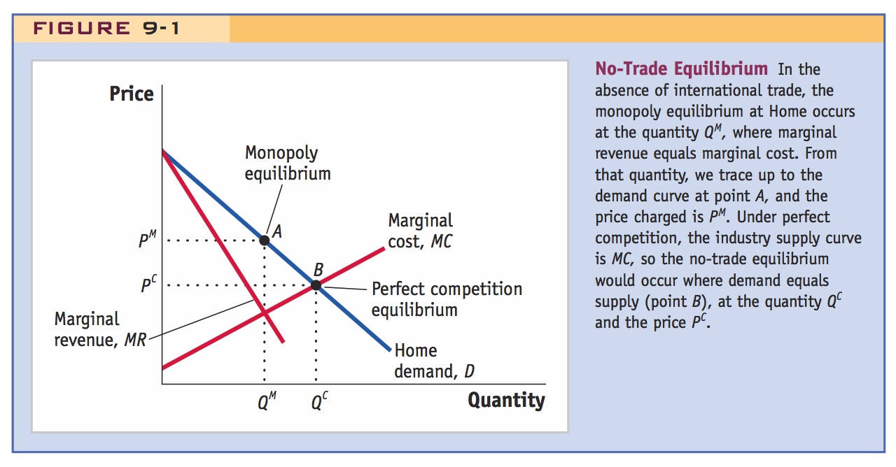
We begin by showing in Figure 9-1 the no-trade equilibrium with a Home monopoly. The Home demand curve is shown by D, and because it is downward-sloping, as the monopolist sells more, the price will fall. This fall in price means that the extra revenue earned by the monopolist from selling one more unit is less than the price: the extra revenue earned equals the price charged for that unit minus the fall in price times the quantity sold of all earlier units. The extra revenue earned from selling one more unit, the marginal revenue, is shown by curve MR in Figure 9-1.
Here again an algebraic example, with linear demand and MC, would fix ideas.
It is now important for MC to be increasing, rather than constant.
To maximize its profits, the monopolist produces at the point where the marginal revenue MR earned from selling one more unit equals the marginal cost MC of producing one more unit. As shown in Figure 9-1, the monopolist produces quantity QM. Tracing up from QM to point A on the demand curve and then over to the price axis, the price charged by the monopolist is PM. This price enables the monopolist to earn the highest profits and is the monopoly equilibrium in the absence of international trade.
This is a traditional comparison, but it raises an interesting issue: It is only legitimate to compare monopoly and perfect competition if demand and costs are identical in both cases. But there might be a good economic reason for the market to be monopolized, so that perfect competition can't be sustained. An example is increasing returns to scale, so there is a natural monopoly. Comparing welfare in the two cases, McCloskey says, is like saying, "if my mother had wheels she would be a tram."
This in turn suggests that it might be interesting to revisit the effects of tariffs and quotas when there is a natural monopoly.
Comparison with Perfect Competition We can contrast the monopoly equilibrium with the perfect competition equilibrium in the absence of trade. Instead of a single firm, suppose there are many firms in the industry. We assume that all these firms combined have the same cost conditions as the monopolist, so the industry marginal cost is identical to the monopolist’s marginal cost curve of MC. Because a perfectly competitive industry will produce where price equals marginal cost, the MC curve is also the industry supply curve. The no-trade equilibrium under perfect competition occurs where supply equals demand (the quantity QC and the price PC). The competitive price PC is less than the monopoly price PM, and the competitive quantity QC is higher than the monopoly quantity QM. This comparison shows that in the absence of trade, the monopolist restricts its quantity sold to increase the market price. Under free trade, however, the monopolist cannot limit quantity and raise price, as we investigate next.
283
Free-Trade Equilibrium
Suppose now that Home engages in international trade. We will treat Home as a “small country,” which means that it faces the fixed world price of PW. In Figure 9-2, we draw a horizontal line at that price and label it as X*, the Foreign export supply curve. At that price, Foreign will supply any quantity of imports (because Home is a small country, the Foreign export supply is perfectly elastic). Likewise, the Home monopolist can sell as much as it desires at the price of PW (because it is able to export at the world price) but cannot charge any more than that price at Home. If it charged a higher price, Home consumers would import the product instead. Therefore, the Foreign supply curve of X* is also the new demand curve facing the Home monopolist: the original no-trade Home demand of D no longer applies.
As an exercise, ask them what would happen if the world price were above the autarky competitive price (but less than the autarky monopoly price).
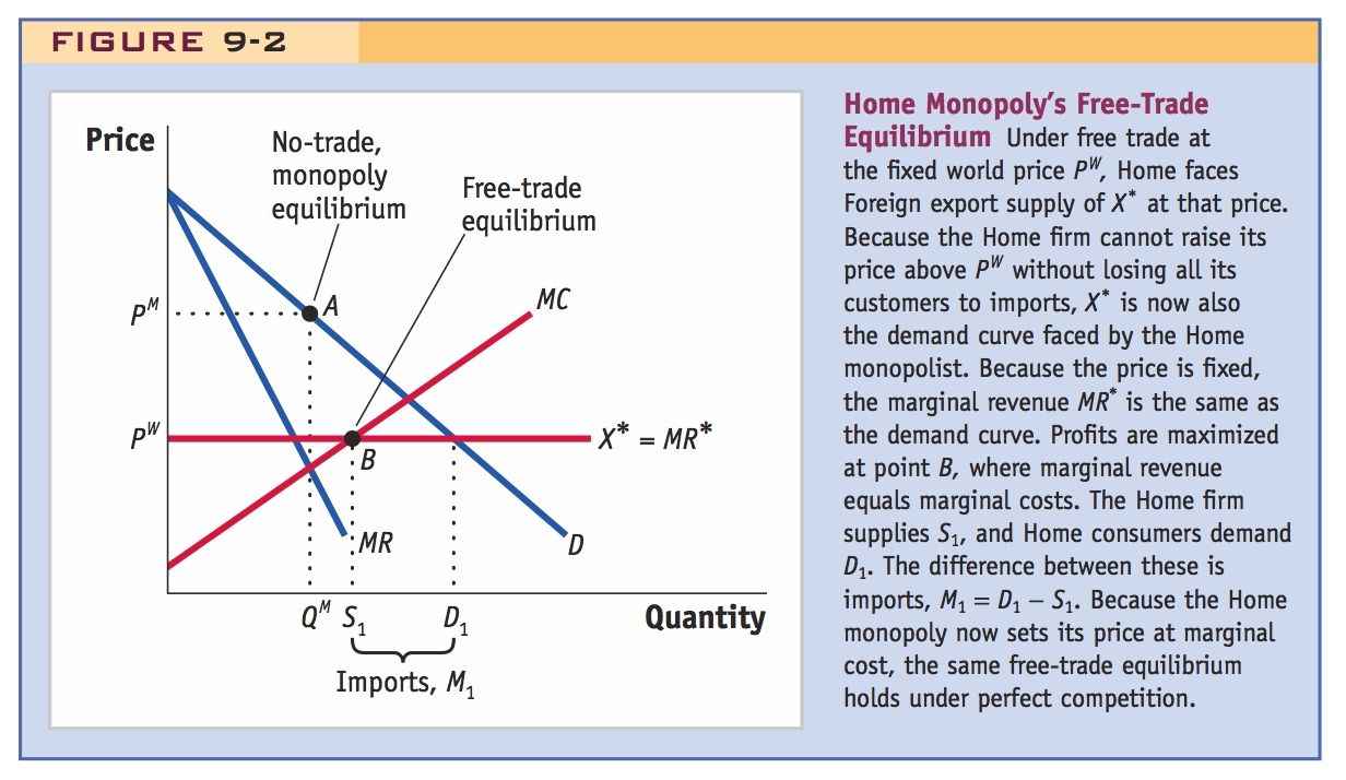
Because this new demand curve facing the Home monopolist is horizontal, the Home firm’s new marginal revenue curve is the same as the demand curve, so X* = MR*. To understand why this is so, remember that marginal revenue equals the price earned from selling one more unit minus the fall in price times the quantity sold of all earlier units. For a horizontal demand curve, there is no fall in price from selling more because additional units sell for PW, the same price for which the earlier units sell. Thus, marginal revenue is the price earned from selling another unit, PW. Therefore, the demand curve X* facing the Home monopolist is identical to the marginal revenue curve; the no-trade marginal revenue of MR no longer applies.
284
Extend the algebraic/numerical example to have an exogenous world price less than the autarky competitive price.
To maximize profits under the new free-trade market conditions, the monopolist will set marginal revenue equal to marginal cost (point B in Figure 9-2) and will supply S1 at the price PW. At the price PW, Home consumers demand D1, which is more than the Home supply of S1. The difference between demand and supply is Home imports under free trade, or M1 = D1 − S1.
The key insight is here: Foreign competition eliminates the firm's market power.
Comparison with Perfect Competition Let us once again compare this monopoly equilibrium with the perfect competition equilibrium, now with free trade. As before, we assume that the cost conditions facing the competitive firms are the same as those facing the monopolist, so the industry supply curve under perfect competition is equal to the monopolist’s marginal cost curve of MC. With free trade and perfect competition, the industry will supply the quantity S1, where the price PW equals marginal cost, and consumers will demand the quantity D1 at the price PW. Under free trade for a small country, then, a Home monopolist produces the same quantity and charges the same price as a perfectly competitive industry. The reason for this result is that free trade for a small country eliminates the monopolist’s control over price; that is, its market power. It faces a horizontal demand curve, equal to marginal revenue, at the world price of PW. Because the monopolist has no control over the market price, it behaves just as a competitive industry (with the same marginal costs) would behave.
So there is an even larger gain from trade.
This finding that free trade eliminates the Home monopolist’s control over price is an extra source of gains from trade for the Home consumers because of the reduction in the monopolist’s market power. We have already seen this extra gain in Chapter 6, in which we first discussed monopolistic competition. There we showed that with free trade, a monopolistically competitive firm faces more-elastic demand curves for its differentiated product, leading it to expand output and lower its prices. The same result holds in Figure 9-2, except that now we have assumed that the good produced by the Home monopolist and the imported good are homogeneous products, so they sell at exactly the same price. Because the Home good and the import are homogeneous, the demand curve X* facing the Home monopolist in Figure 9-2 is perfectly elastic, leading the monopolist to behave in the same way under free trade as in a competitive industry.
Effect of a Home Tariff
Now suppose the Home country imposes a tariff of t dollars on imports, which increases the Home price from PW to PW + t. In Figure 9-3, the effect of the tariff is to raise the Foreign export supply curve from X* to X* + t. The Home firm can sell as much as it desires at the price of PW + t but cannot charge any more than that price. If it did, the Home consumers would import the product. Thus, the Foreign supply curve of X* + t is also the new demand curve facing the Home monopolist.
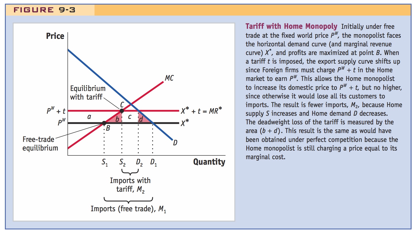
Because this new demand curve is horizontal, the new marginal revenue curve is once again the same as the demand curve, so MR* = X* + t. The reasoning for this result is similar to the reasoning under free trade: with a horizontal demand curve, there is no fall in price from selling more, so the Home firm can sell as much as it desires at the price of PW + t. So the demand curve X* + t facing the Home monopolist is identical to its marginal revenue curve.
285
To maximize profits, the monopolist will once again set marginal revenue equal to marginal costs, which occurs at point C in Figure 9-3, with the price PW + t and supply of S2. At the price PW + t, Home consumers demand D2, which is more than Home supply of S2. The difference between demand and supply is Home imports, M2 = D2 − S2. The effect of the tariff on the Home monopolist relative to the free-trade equilibrium is to raise its production from S1 to S2 and its price from PW to PW + t. The supply increase in combination with a decrease in Home demand reduces imports from M1 to M2.
Since the monopolist has lost its market power, the effect of the tariff must ipso facto be the same as in a competitive industry.
Comparison with Perfect Competition Let us compare this monopoly equilibrium with the tariff to what would happen under perfect competition. The tariff-inclusive price facing a perfectly competitive industry is PW + t, the same price faced by the monopolist. Assuming that the industry supply curve under perfect competition is the same as the monopolist’s marginal cost MC, the competitive equilibrium is where price equals marginal cost, which is once again at the quantity S2 and the price PW + t. So with a tariff, a Home monopolist produces the same quantity and charges the same price as would a perfectly competitive industry. This result is similar to the result we found under free trade. This similarity occurs because the tariff still limits the monopolist’s ability to raise its price: it can raise the price to PW + t but no higher because otherwise consumers will import the product. Because the monopolist has limited control over its price, it behaves in the same way a competitive industry would when facing the tariff.
Home Loss Due to the Tariff Because the tariff and free-trade equilibria are the same for a Home monopoly and a perfectly competitive industry, the deadweight loss from the tariff is also the same. As we learned in the previous chapter, the deadweight loss under perfect competition is found by taking the total fall in consumer surplus due to the rise in price from PW to PW + t, adding the gain in producer surplus from the rise in price, and then adding the increase in government revenue due to the tariff. Summing all these components shows a net welfare loss of (b + d):
286
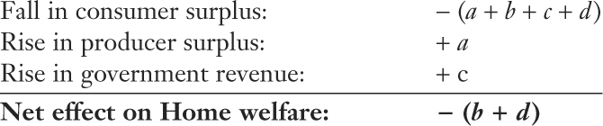
Under Home monopoly, the deadweight loss from the tariff is the same. Home consumers still have the loss of (a + b + c + d) because of the rise in price, while the Home monopolist gains the amount a in profits because of the rise in price. With the government collecting area c in tariff revenue, the deadweight loss is still area (b + d).
Effect of a Home Quota
Before getting into the details, emphasize this intuition and explain why the result matters to the ITO.
Let us now contrast the tariff with an import quota imposed by the Home government. As we now show, the quota results in a higher price for Home consumers, and therefore a larger Home loss, than would a tariff imposed on the same equilibrium quantity of imports. The reason for the higher costs is that the quota creates a “sheltered” market for the Home firm, allowing it to exercise its monopoly power, which leads to higher prices than under a tariff. Economists and policy makers are well aware of this additional drawback to quotas, which is why the WTO has encouraged countries to replace many quotas with tariffs.
To show the difference between the quota and tariff with a Home monopoly, we use Figure 9-4, in which the free-trade equilibrium is at point B and the tariff equilibrium is at point C (the same points that appear in Figure 9-3). Now suppose that instead of the tariff, a quota is applied. We choose the quota so that it equals the imports under the tariff, which are M2. Since imports are fixed at that level, the effective demand curve facing the Home monopolist is the demand curve D minus the amount M2. We label this effective demand curve D − M2. Unlike the situation under the tariff, the monopolist now retains the ability to influence its price: it can choose the optimal price and quantity along D − M2. We graph the marginal revenue curve MR for the effective demand curve D − M2. The profit-maximizing position for the monopolist is where marginal revenue equals marginal cost, at point E, with price P3 and supply S3.
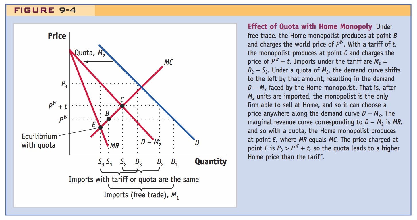
Let us now compare the tariff equilibrium, at point C, with the quota equilibrium, at point E. It will definitely be the case that the price charged under the quota is higher, P3 > PW + t. The higher price under the quota reflects the ability of the monopolist to raise its price once the quota amount has been imported. The higher price occurs even though the quota equilibrium has the same level of imports as the tariff, M2. Therefore, the effects of a tariff and a quota are no longer equivalent as they were under perfect competition: the quota enables a monopolist to exercise its market power and raise its price.
What about the quantity produced by the monopolist? Because the price is higher under the quota, the monopolist will definitely produce a lower quantity under the quota, S3 < S2. What is more surprising, however, is that it is even possible that the quota could lead to a fall in output as compared with free trade: in Figure 9-4, we have shown S3 < S1. This is not a necessary result, however, and instead we could have drawn the MR curve so that S3 > S1. It is surprising that the case S3 < S1 is even possible because it suggests that workers in the industry would fail to be protected by the quota; that is, employment could fall because of the reduction in output under the quota. We see, then, that the quota can have undesirable effects as compared with a tariff when the Home industry is a monopoly.
287
Key result.
Home Loss Due to the Quota Our finding that Home prices are higher with a quota than with a tariff means that Home consumers suffer a greater fall in surplus because of the quota. On the other hand, the Home monopolist earns higher profit from the quota because its price is higher. We will not make a detailed calculation of the deadweight loss from the quota with Home monopoly because it is complicated. We can say, however, that the deadweight loss will always be higher for a quota than for a tariff because the Home monopolist will always charge a higher price. That higher price benefits the monopolist but harms Home consumers and creates an extra deadweight loss because of the exercise of monopoly power.
Furthermore, the fact that the Home monopolist is charging a higher price also increases the quota rents, which we defined in the previous chapter as the ability to import goods at the world price and sell them at the higher Home price (in our example, this is the difference between P3 and PW times the amount of imports M2). In the case of Home monopoly, the quota rents are greater than government revenue would be under a tariff. Recall that quota rents are often given to Foreign countries in the case of “voluntary” export restraints, when the government of the exporting country implements the quota, or else quota rents can even be wasted completely when rent-seeking activities occur. In either of these cases, the increase in quota rents adds to Home’s losses if the rents are given away or wasted.
In the next application, we examine a quota used in the United States during the 1980s to restrict imports of Japanese cars. Because the car industry has a small number of producers, it is imperfectly competitive. So our predictions from the case of monopoly discussed previously can serve as a guide for what we expect in the case of Home oligopoly.
288
Japan implements a VER on U.S. autos in 1981 to avoid threatened U.S. quotas. U.S. car prices increased. Quota rents to Japanese firms were at least $2.2 billion. VERs were exempted from the prohibition of quotas in GATT, but this loophole was closed by the WTO in 1995.
This was the period over which the dollar was appreciating, which created unprecedented political pressure on Congress in favor of protectionist policies.
In fact, they happily volunteered to extend them after the agreement lapsed.
U.S. Imports of Japanese Automobiles
A well-known case of a “voluntary” export restraint (VER) for the United States occurred during the 1980s, when the U.S. limited the imports of cars from Japan. To understand why this VER was put into place, recall that during the early 1980s, the United States suffered a deep recession. That recession led to less spending on durable goods (such as automobiles), and as a result, unemployment in the auto industry rose sharply.
In 1980 the United Automobile Workers and Ford Motor Company applied to the International Trade Commission (ITC) for protection under Article XIX of the General Agreement on Tariffs and Trade (GATT) and Section 201 of U.S. trade laws. As described in the previous chapter, Section 201 protection can be given when increased imports are a “substantial cause of serious injury to the domestic industry,” where “substantial cause” must be “not less than any other cause.” In fact, the ITC determined that the U.S. recession was a more important cause of injury to the auto industry than increased imports. Accordingly, it did not recommend that the auto industry receive protection.
With this negative determination, several members of Congress from states with auto plants continued to pursue import limits by other means. In April 1981 Senators John Danforth from Missouri and Lloyd Bentsen from Texas introduced a bill in the U.S. Senate to restrict imports. Clearly aware of this pending legislation, the Japanese government announced on May 1 that it would “voluntarily” limit Japan’s export of automobiles to the U.S. market. For the period April 1981 to March 1982, this limit was set at 1.83 million autos. After March 1984 the limit was raised to 2.02 million and then to 2.51 million vehicles annually. By 1988 imports fell below the VER limit because Japanese companies began assembling cars in the United States.
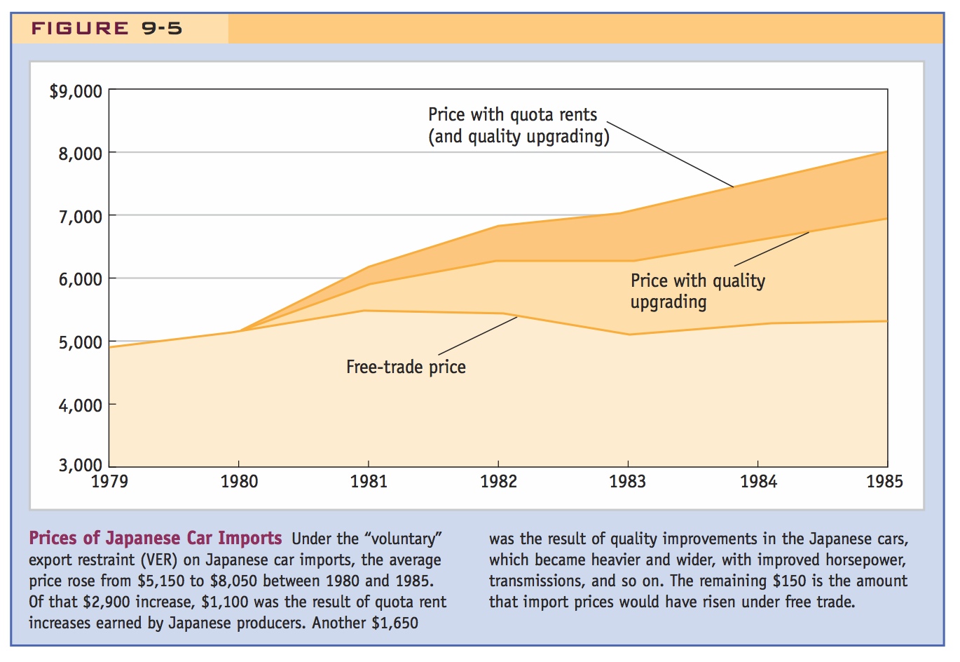
We are interested in whether American producers were able to exercise their monopoly power and raise their prices under the quota restriction. We are also interested in how much import prices increased. To measure the increase in import prices, we need to take into account a side effect of the 1980 quota: it led to an increase in the features of Japanese cars being sold in the United States such as size, weight, horsepower, and so on, or what we call an increase in quality.3 The overall increase in auto import prices during the 1980s needs to be broken up into the increases due to (1) the quality upgrading of Japanese cars; (2) the “pure” increase in price because of the quota, which equals the quota rents; and (3) any price increase that would have occurred anyway, even if the auto industry had not been subject to protection.
Price and Quality of Imports The impact of the VER on the price of Japanese cars is shown in Figure 9-5. Under the VER on Japanese car imports, the average price rose from $5,150 to $8,050 between 1980 and 1985. Of that $2,900 increase, $1,100 was the result of quota rents earned by Japanese producers in 1984 and 1985. Another $1,650 was from quality improvements in the Japanese cars, which became heavier and wider, with improved horsepower, transmissions, and so on. The remaining $150 is the amount that import prices would have risen under free trade.
289
Quota Rents If we multiply the quota rents of $1,100 per car by the imports of about 2 million cars, we obtain total estimated rents of $2.2 billion, which is the lower estimate of the annual cost of quota rents for automobiles. The upper estimate of $7.9 billion comes from also including the increase in price for European cars sold in the United States. Although European cars were not restricted by a quota, they did experience a significant increase in price during the quota period; that increase was due to the reduced competition from Japanese producers.
The Japanese firms benefited from the quota rents that they received. In fact, their stock prices rose during the VER period, though only after it became clear that the Japanese Ministry of International Trade and Industry would administer the quotas to each producer (so that the Japanese firms would capture the rents). Moreover, because each producer was given a certain number of cars it could export to the United States, but no limit on the value of the cars, producers had a strong incentive to export more expensive models. That explains the quality upgrading that occurred during the quota, which was when Japanese producers started exporting more luxurious cars to the United States.
290
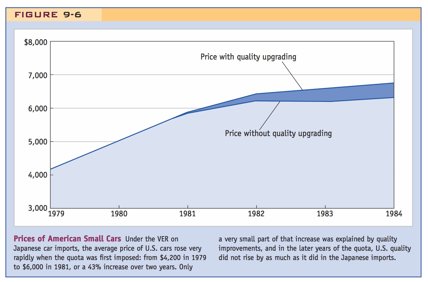
Price of U.S. Cars What happened to the prices of American small cars during this period? Under the VER on Japanese car imports, the average price of U.S. cars rose very rapidly when the quota was first imposed: from $4,200 in 1979 to $6,000 in 1981, a 43% increase over two years. That price increase was due to the exercise of market power by the U.S. producers, who were sheltered by the quota on their Japanese competitors. Only a small part of that price increase was explained by quality improvements since the quality of U.S. cars did not rise by as much as the quality of Japanese imports, as seen in Figure 9-6. So the American producers were able to benefit from the quota by raising their prices, and the Japanese firms also benefited by combining a price increase with an improvement in quality. The fact that both the Japanese and U.S. firms were able to increase their prices substantially indicates that the policy was very costly to U.S. consumers.
The GATT and WTO The VER that the United States negotiated with Japan in automobiles was outside of the GATT framework: because this export restraint was enforced by the Japanese rather than the United States, it did not necessarily violate Article XI of the GATT, which states that countries should not use quotas to restrict imports. Other countries used VERs during the 1980s and early 1990s to restrict imports in products such as automobiles and steel. All these cases were exploiting a loophole in the GATT agreement whereby a quota enforced by the exporter was not a violation of the GATT. This loophole was closed when the WTO was established in 1995. Part of the WTO agreement states that “a Member shall not seek, take or maintain any voluntary export restraints, orderly marketing arrangements or any other similar measures on the export or the import side. These include actions taken by a single Member as well as actions under agreements, arrangements and understandings entered into by two or more Members.”4 As a result of this rule, VERs can no longer be used unless they are a part of some other agreement in the WTO.5
291
The bottom line
Suggest mentioning this first, to explain why the U.S. and Japan were able to resort to quotas at all.