674

Now that we have reviewed greenhouse gases and their role in global warming, we can explore the evidence that an increased concentration of greenhouse gases is causing Earth to become warmer. If Earth is becoming warmer, we can begin to evaluate whether or not this warming is caused by human activities that have released greenhouse gases. One way to make these assessments is to determine gas concentrations and temperatures from the past and compare them to gas concentrations and temperatures in the present day. We can also use information about changes in gas concentrations and temperatures to predict future climate conditions. In this module, we will examine how greenhouse gas concentrations have changed over time and how these changes are linked to global warming.

Learning Objectives

After reading this module you should be able to

In 1988 the United Nations and the World Meteorological Organization created the Intergovernmental Panel on Climate Change (IPCC), a group of more than 3,000 scientists from around the world working together to assess climate change. Their mission is to understand the details of the global warming system, the effects of climate change on biodiversity and energy fluxes in ecosystems, and the economic and social effects of climate change. The IPCC enables scientists to assess and communicate the state of our knowledge and to suggest research directions that would improve our understanding in the future. This effort has produced an excellent understanding of how greenhouse gases and temperatures are linked.

Measuring CO₂ Concentrations in the Atmosphere

675

Through the work of the IPCC, we now understand that CO₂ is an important greenhouse gas that can contribute to global warming, but we didn’t always realize this. In the first half of the twentieth century, most scientists believed that if any excess CO₂ were being produced, it would be absorbed by the oceans and vegetation. In addition, because the concentration of atmospheric CO₂ was low compared to gases such as oxygen and nitrogen, it was difficult to measure accurately.

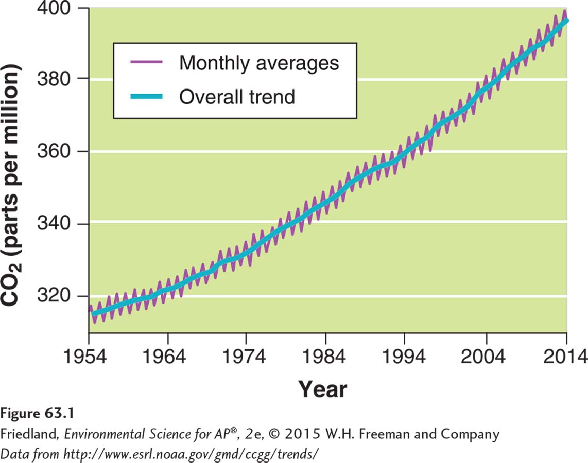
Charles David Keeling was the first to overcome the technical difficulties in measuring CO₂. When Keeling set out to measure the precise level of CO₂ in the atmosphere, most atmospheric scientists believed that two measurements several years apart would be sufficient to answer the question of whether human activities were causing increased concentrations of CO₂ in the atmosphere. Keeling did not agree and in 1958 he began collecting data throughout the year at the Mauna Loa Observatory in Hawaii. After just 1 year of work, Keeling found that CO₂ levels varied seasonally and that the concentration of CO₂ increased from year to year. His results prompted him to take measurements for several more years, and he and his students have continued this work into the twenty-first century. The results, shown in FIGURE 63.1, confirm Keeling’s early findings; although CO₂ concentrations vary between seasons, there is a clear trend of rising CO₂ concentrations across the years. This increase over time is correlated to increased human emissions of carbon from the combustion of fossil fuels and net destruction of vegetation. “Do the Math: Projecting Future Increases in CO₂” gives you an opportunity to estimate the increase in CO₂ concentrations by the end of the century.

What causes the seasonal variation? Each spring, as deciduous trees, grasslands, and farmlands in the Northern Hemisphere turn green, they increase their absorption rates of CO₂ to carry out photosynthesis. At the same time, bodies of water begin to warm and the algae and plants also begin to photosynthesize. In doing so, these producers take up some of the CO₂ in the atmosphere. Conversely, in the fall, as leaves drop, crops are harvested, and bodies of water cool, the uptake of atmospheric CO₂ by algae and plants declines and the amount of CO₂ in the atmosphere increases.

CO₂ Emissions Differ Among Nations

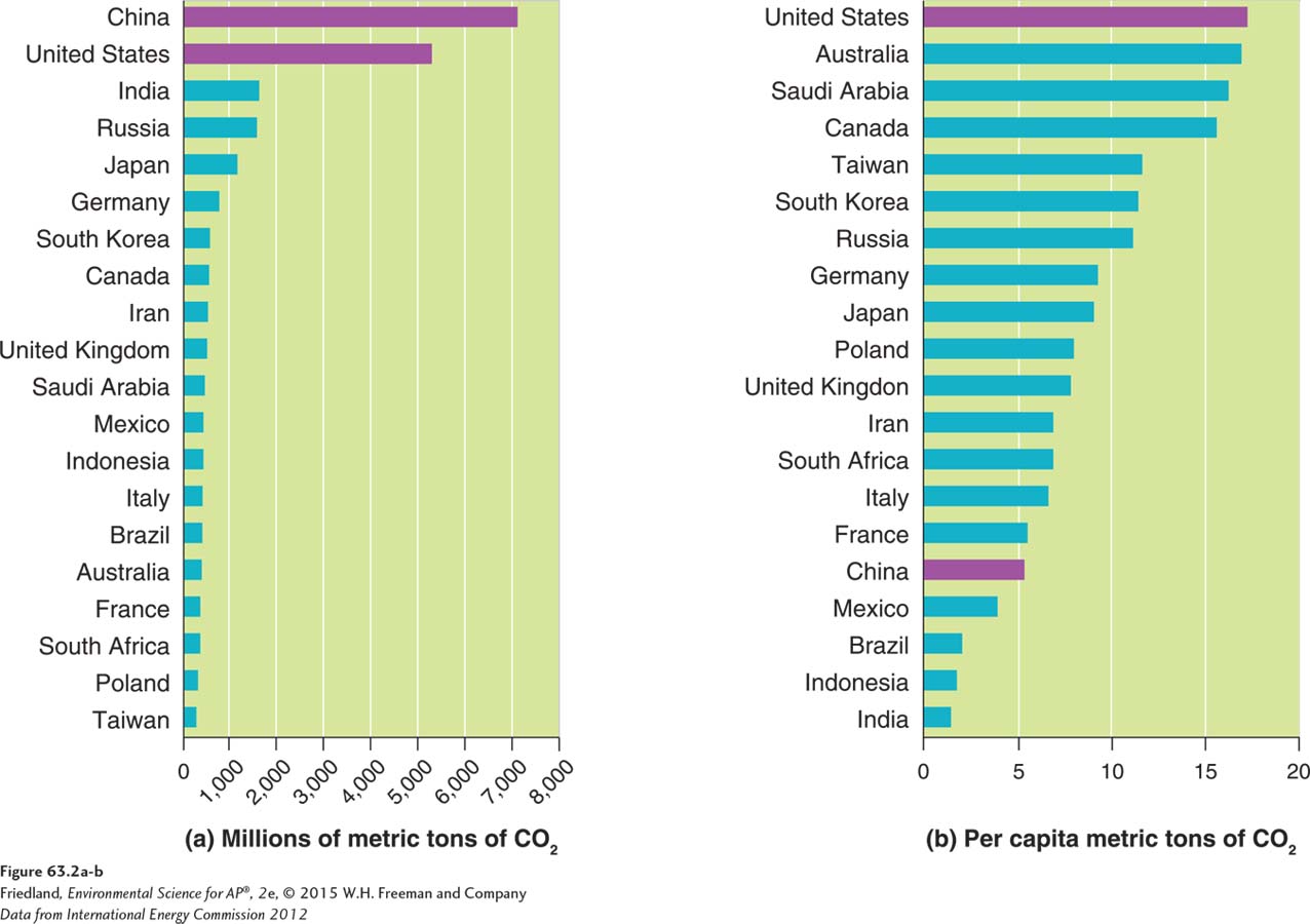
Throughout this book we have seen that per capita consumption of fossil fuel and materials is greatest in developed countries. It is not surprising, then, that the production of carbon dioxide has also been greatest in the developed world. For many decades, the 20 percent of the population living in the developed world—roughly 1 billion people—produced about 75 percent of the carbon dioxide. However, these percentages are changing as some developing nations industrialize and acquire more vehicles that burn fossil fuels. In 2009, developing countries surpassed developed countries in the production of CO₂.

Development has been especially rapid in China and India, which together contain one-third of the world’s population. From 2000 to 2009, China more than doubled its emissions of carbon dioxide as the country built many new coal-powered electrical plants that increased its ability to burn coal. FIGURE 63.2a, shows that today China is the leading emitter of CO₂. China emits more than 7,200 million metric tons of CO₂, representing 24 percent of all global CO₂ emissions. The United States is in second place, emitting more than 5,300 million metric tons. This represents 18 percent of all global CO₂ emissions, yet the United States contains only 5 percent of the world’s population. If we consider the amount of per capita CO₂ emissions, shown in FIGURE 63.2b, we obtain a very different picture of which countries produce the most CO₂. The United States and Australia are the leading per capita emitters of CO₂, followed by Saudi Arabia and Canada. Despite the fact that China and India rank among the top producers of CO₂, their per capita production ranks them sixteenth and twentieth, respectively, which reflects the fact that these two countries both have very large populations.

677

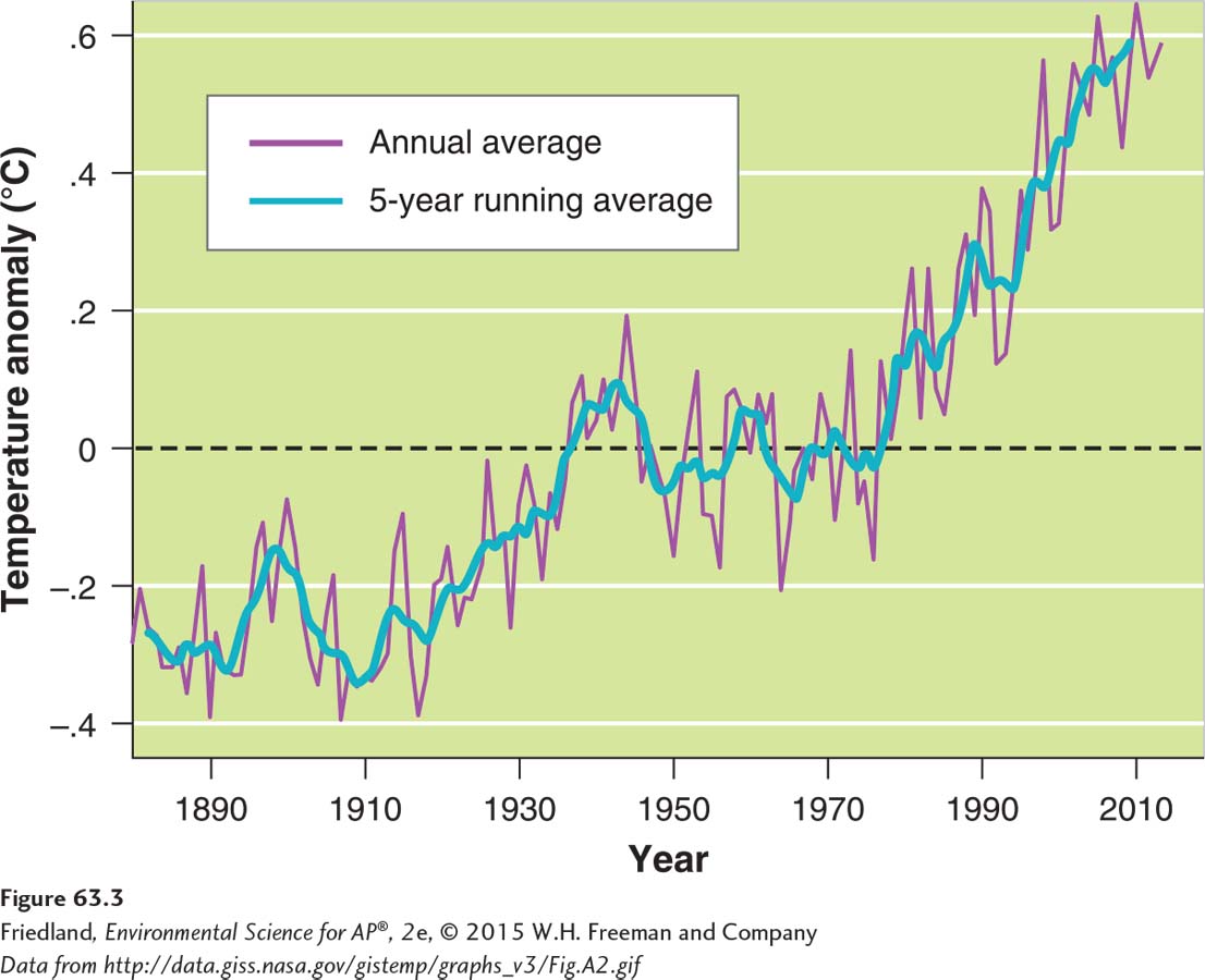
Before we can determine if global temperature increases are a recent phenomenon and if these increases are unusual, we must establish how the temperatures of Earth have changed in the past. Since about 1880, there have been enough direct measurements of land and ocean temperatures that the NASA Goddard Institute for Space Studies has been able to generate a graph of global temperature change over time. This graph, updated monthly, is shown in FIGURE 63.3. Comprising thousands of measurements from around the world, the graph shows global temperatures have increased 0.8°C (1.4°F) from 1880 through 2013. In fact, the 10 warmest years on record since 1880 have all occurred between 1998 and 2013.

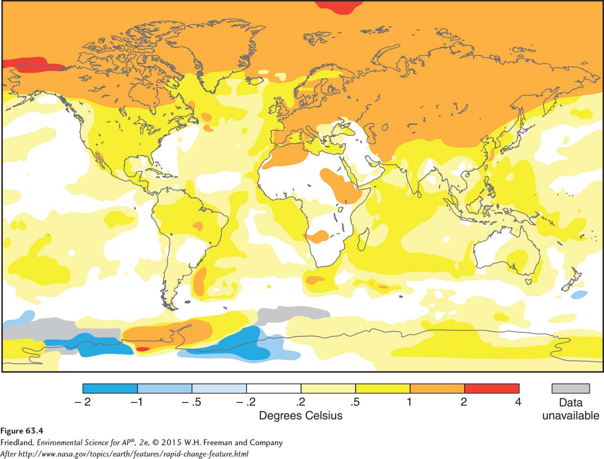
While an increase in average global temperature of 0.8°C (1.4°F) may not sound very substantial, it not evenly distributed around the globe. As the map in FIGURE 63.4 shows, some regions, including parts of Antarctica, have experienced cooler temperatures. Some regions, including areas of the oceans, have experienced no change in temperature. Finally, some regions, such as those in the extreme northern latitudes, have experienced increases of 1°C to 4°C (1.8°F –7.2°F). The substantial increases in temperatures in the northern latitudes have caused, among other problems, nearly 45 percent of the northern ice cap to melt, which has threatened polar bears and their ecosystem, as discussed at the beginning of this chapter.

The data collected by the NASA clearly demonstrate that the globe has been slowly warming during the past 120 years. However, it is possible that such changes in temperature are simply a natural phenomenon. If we want to know whether these changes are typical, we must examine a much longer span of time.

Since no one was measuring temperatures thousands of years ago, we must use indirect measurements. Common indirect measurements include changes in the species composition of organisms that have been preserved over millions of years and chemical analyses of air bubbles formed in ice long ago.

Changing Species Compositions

One commonly used biological measurement is the change in species composition of a group of small protists, called foraminifera. Foraminifera are tiny, marine organisms with hard shells that resist decay after death (FIGURE 63.5). In some regions of the ocean floor, the tiny shells have been building up in sediments for millions of years. The youngest sediment layers are near the top of the ocean floor whereas the oldest sediment layers are much deeper. Fortunately, different species of foraminifera prefer different water temperatures. As a result, when scientists identify the predominant species of foraminifera in a layer of sediment, they can infer the likely temperature of the ocean at the time the layer of sediment was deposited. By examining thousands of sediment layer samples, we can gain insights into temperature changes over millions of years.

678

Air Bubbles in Ancient Ice

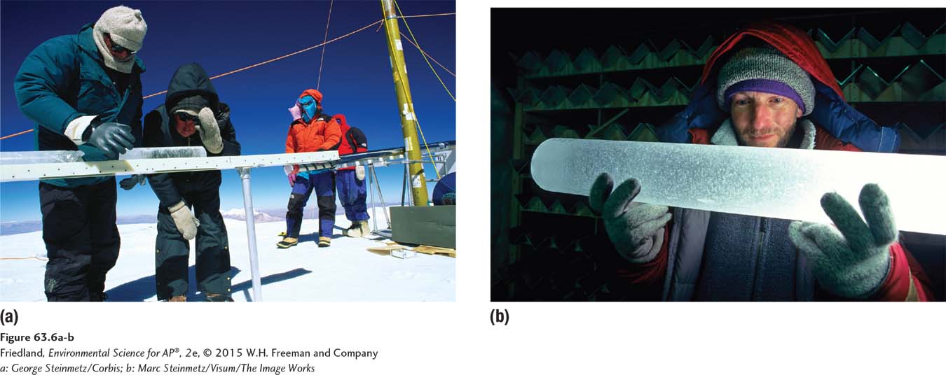
Scientists can determine changes in greenhouse gas concentrations and temperatures over long periods of time by examining ancient ice. In cold areas such as Antarctica and at the top of the Himalayas, the snowfall each year eventually compresses to become ice. Similar to marine sediments, the youngest ice is near the surface and the oldest ice is much deeper. During the process of compression, the ice captures small air bubbles. These bubbles contain tiny samples of the atmosphere that existed at the time the ice was formed. Scientists have traveled to these frozen regions of the world to drill deep into the ice and extract long tubes of ice called ice cores (FIGURE 63.6). Samples of ice cores can span up to 500,000 years of ice formation. Scientists determine the age of different layers in the ice core and then melt the ice from a piece associated with a particular time period. When the piece of ice melts, air bubbles are released and scientists measure the concentration of greenhouse gases in the air when the bubbles were trapped in the ancient ice.

679

Oxygen atoms in melted ice cores can also be used to determine temperatures from the distant past. Oxygen atoms occur in two forms, or isotopes: light oxygen, also known as oxygen-16 (¹⁶O), contains 8 protons plus 8 neutrons. In contrast, heavy oxygen, also known as oxygen-18 (¹⁸O), contains 8 protons plus 10 neutrons. Ice formed during a period of warmer temperatures contains a higher percentage of heavy oxygen than ice formed during colder temperatures. By examining changes in the percentage of heavy oxygen atoms from different layers of the ice core, we can indirectly estimate temperatures from hundreds of thousands of years ago.

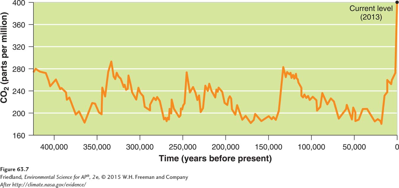
Combining data from different biological and physical measurements, researchers have created a picture of how the atmosphere and temperature of Earth have changed over hundreds of thousands of years. FIGURE 63.7 shows the pattern of atmospheric CO₂. Notice that for over 400,000 years, the atmosphere never contained more than 300 ppm of CO₂. In contrast, from 1958 to 2013 the concentration of CO₂ in the atmosphere has rapidly climbed from 310 to 400 ppm. This means that the rise of CO₂ in the atmosphere during the past 50 years is unprecedented.

680

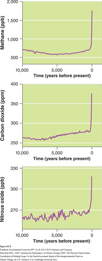
During the past 10,000 years, CO₂ is not the only greenhouse gas whose concentration has increased. As you can see in FIGURE 63.8, methane and nitrous oxide show a pattern of increase that is similar to the pattern we saw for CO₂. For all three gases, there was little change in concentration for most of the previous 10,000 years. After 1800, however, concentrations of the three gases all rose dramatically. Given what we now know about the anthropogenic sources of greenhouse gases, this increase in greenhouse gases occurred because this time period marks the start of the Industrial Revolution when humans began burning large amounts of fossil fuel and producing a variety of greenhouse gases.

FIGURE 63.9 charts historic temperatures and CO₂ concentrations. Looking at the blue line, we see that temperatures have changed dramatically over the past 400,000 years. Most of these rapid shifts occurred during the onset of an ice age or during the transition from an ice age to a period of warm temperatures after an ice age. Because these changes occurred before humans could have had an appreciable effect on global systems, scientists suspect the changes were caused by small, regular shifts in the orbit of Earth. The path of the orbit, the amount of tilt on Earth’s axis, and the position relative to the Sun all change regularly over hundreds of thousands of years. These changes alter the amount of sunlight that hits high northern latitudes in the winter, the amount of snow that can accumulate, and the way the albedo effect keeps energy from being absorbed and converted to heat. These changes could give rise to fairly regular shifts in temperature over a long period of time.

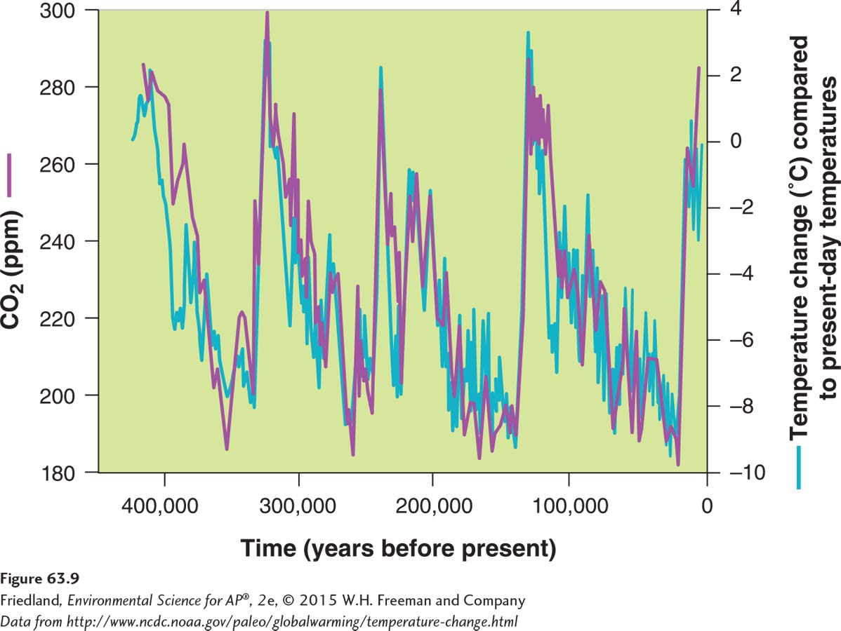
The more important insight from FIGURE 63.9 is the close correspondence between historic temperatures and CO₂ concentrations. But the graph does not tell us the nature of this relationship. Did periods of increased CO₂ cause increased temperature; did periods of increased temperature cause increased production of CO₂; or is another factor at work? Scientists believe that the relationship between fluctuating levels of CO₂ and the temperature is complex and that both factors play a role. As we know, the increase of CO₂ in the atmosphere causes a greater capacity for warming through the greenhouse effect. However, when Earth experiences higher temperatures, the oceans warm and cannot contain as much CO₂ gas and, as a result, they release CO₂ into the atmosphere. What ultimately matters is the net movement of CO₂ between the atmosphere and the oceans and how these different feedback loops work together to affect global temperatures.

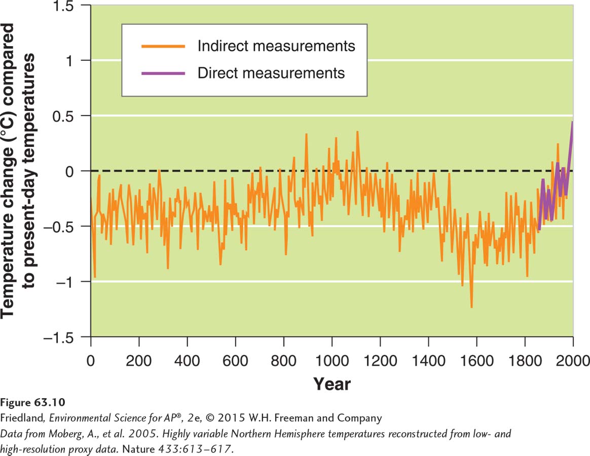
We can also examine temperatures over somewhat shorter time periods. For example, scientists have used indirect and direct measures to determine global temperatures during the past 2,000 years. They then selected the average temperature from 1901 to 2000 as a baseline against which all other years can be compared. FIGURE 63.10 shows that average temperature from 0 CE to 800 CE was cooler than the average measured during the twentieth century. Temperatures then tended to warm during 800 CE to 1200 CE and cooler from 1500 to 1800. It is particularly striking that the change in temperature during the past century has increased rapidly and that the average temperatures that we are experiencing today are higher than those experienced in the past 2,000 years.

681

Greenhouse Gases versus Increased Solar Radiation

We have seen that the surface temperature of Earth has increased roughly 0.8°C (1.4°F) over the past 120 years. But larger changes in temperature have occurred over the past 400,000 years without human influence. How can we tell if the recent changes are anthropogenic? One explanation for warming temperatures during the past century is an increase in solar radiation. Another possibility is that warming is caused by increased CO₂ in addition to warming caused by natural fluctuations in solar radiation. In other words, both factors might be important. Unfortunately, simply looking at temperature and CO₂ data averages around the globe will not allow us to determine if either of these two possibilities is correct.

682

One way to approach the problem is to look for more detailed patterns in temperature changes. For example, if increased CO₂ concentrations caused global warming by preventing heat loss, then periods of elevated CO₂ would be associated with higher temperatures more commonly in winter than in summer, at night rather than during the day, and in the Arctic rather than in warmer latitudes. These three scenarios are all associated with colder temperatures, so reducing heat loss would have a bigger impact on temperature than in scenarios in which the temperatures were already quite warm. In fact, we already observed this when we examined the changes in temperature around the world in FIGURE 63.4—the Arctic regions are experiencing the greatest amount of warming.

On the other hand, if increased solar radiation were the cause of global warming, periods of elevated solar radiation would be associated with higher temperatures more commonly when the Sun is shining more—namely in the summer, during the day, and at low latitudes. These times and locations on Earth receive the greatest amount of sunlight, so an increased intensity of solar radiation would cause these times and places on Earth to warm more than other times and places. When scientists make these types of detailed comparisons, they find that the patterns in temperature change are strongly consistent with increased greenhouse gases such as CO₂ and not consistent with increased solar radiation. This body of evidence led the IPCC to conclude in 2007 that most of the observed increase in global average temperatures since the mid-twentieth century has been the result of increased concentrations of anthropogenic greenhouse gas.

Climate Models and the Prediction of Future Global Temperatures

Just as indirect indicators can help us get a picture of what the temperature has been in the distant past, computer models can help us predict future climate conditions. Researchers can determine how well a model approximates real-world processes by applying it to a time in the past for which we have accurate data on conditions such as air and ocean temperatures, CO₂ concentration, extent of vegetation, and sea ice coverage at the poles. Modern models reproduce recent temperature fluctuations well over large spatial scales. From this work modelers are fairly confident that climate models capture the most significant features of today’s climate.

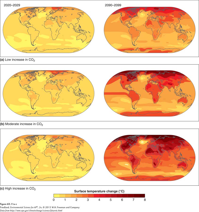
Although climate models cannot forecast future climates with total accuracy, as the models improve scientists have been able to place more confidence in their predictions of temperature change, although they have had more difficulty predicting changes in precipitation. Because assumptions vary among different climate models, when multiple models predict similar changes, we can have increased confidence that the predictions are robust. FIGURE 63.11 shows recent predictions based on the data from climate models. Scientists generally agree that average global temperatures will rise by 1.8°C to 4°C (3.2°F–7.2°F) by the year 2100, depending on whether CO₂ emissions experience slow, moderate, or high growth over time.

The global greenhouse system is made up of several interconnected subsystems with many potential positive and negative feedbacks. As we saw in Chapter 2 with population systems, positive feedbacks amplify changes. Because of this, positive feedback often leads to an unstable situation in which small fluctuations in inputs lead to large observed effects. On the other hand, negative feedbacks dampen changes. When we think about how anthropogenic greenhouse gases will affect Earth, we must ask whether positive or negative feedbacks will predominate. We do not currently have enough evidence to settle this question conclusively, but we can examine some of the feedback cycles and the way they influence temperatures on Earth.

Positive Feedbacks

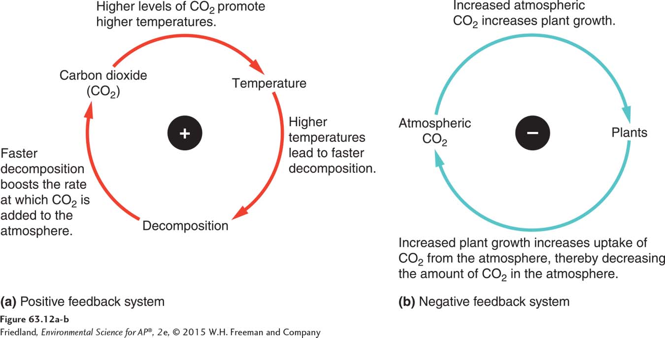
There are many ways that a rise in temperatures could create a positive feedback. For example, global soils contain more than twice as much carbon as the amount currently in the atmosphere. As shown in FIGURE 63.12a, higher temperatures are expected to increase the biological activity of decomposers in these soils. Because this decomposition leads to the release of additional CO₂ from the soil into the atmosphere, the temperature change will be amplified even more.

A similar, but more troubling, scenario is expected in tundra biomes containing permafrost. As atmospheric concentrations of CO₂ from anthropogenic sources increase, the Arctic regions become substantially warmer and the frozen tundra begins to thaw. As it thaws, the tundra develops areas of standing water with little oxygen available under the water as the thick organic layers of the tundra begin to decompose. As a result, the organic material experiences anaerobic decomposition that produces methane, a stronger greenhouse gas than CO₂, which should lead to even more global warming.

683

Negative Feedbacks

One of the most important negative feedbacks occurs as plants respond to increases in atmospheric carbon. FIGURE 63.12b shows this cycle. Because carbon dioxide is required for photosynthesis, an increase in CO₂ can stimulate plant growth. The growth of more plants will cause more CO₂ to be removed from the atmosphere. This negative feedback, which causes carbon dioxide and temperature increases to be smaller than they otherwise would have been, appears to be one of the reasons why only about half of the CO₂ emitted into the atmosphere by human activities has remained in the atmosphere.

684

A second negative feedback exists in the oceans. As CO₂ concentrations increase in the atmosphere, more CO₂ is absorbed by the oceans. Although this is beneficial because it reduces CO₂ in the atmosphere, it causes harmful effects to the oceans. When CO₂ dissolves in water, much of it combines with water molecules to form carbonic acid (H₂CO₃). Since this is an equilibrium reaction, an increase in ocean CO₂ causes more CO₂ to be converted to carbonic acid, which lowers the pH of the water in a process known as ocean acidification. Ocean acidification is of particular concern for the wide variety of species that build shells and skeletons made of calcium carbonate, including corals, mollusks, and crustaceans. As pH decreases, the calcium carbonate in these organisms can begin to dissolve and the ocean’s saturation point for calcium carbonate declines, which makes it harder for organisms to acquire the material they need to build their shells and skeletons.

The Limitations of Feedbacks

Most of the feedbacks we have discussed are limited by features of the systems in which they take place. For example, the soil-carbon feedback is limited by the amount of carbon in soils. While warming soils could add large amounts of CO₂ to the atmosphere for a time, eventually soil stocks will become so low that biological activity falls back to earlier rates. The enhanced CO₂ uptake by plants is also limited: Studies indicate that only some plants benefit from CO₂ fertilization, and often the growth is enhanced only until another factor becomes limiting, such as water or nutrients.

The magnitude and direction of many feedbacks are complex. For example, water vapor has both positive and negative feedbacks and there are limits to each. As temperatures increase, water can evaporate into the atmosphere more easily. Because water vapor is an important greenhouse gas, this increased evaporation will lead to further warming. There is a limit, however, to the amount of water vapor that can exist in the air. As we discussed in Chapter 4, air can become saturated with water vapor and the amount of saturation changes with temperature. Increased water vapor in the atmosphere can lead to the formation of clouds that can shield the surface of Earth from solar radiation, leading to a negative feedback. In short, the net effect of water vapor on global temperatures depends on several simultaneously occurring processes that make predictions difficult.