module 19 Population Growth Models
196
Scientists often use models to help them explain how things work and to predict how things might change in the future. Population ecologists use growth models that incorporate density-
Learning Objectives
After reading this module you should be able to
explain the exponential growth model of populations, which produces a J-
shaped curve. describe how the logistic growth model incorporates a carrying capacity and produces an S-
shaped curve. compare the reproductive strategies and survivorship curves of different species.
explain the dynamics that occur in metapopulations.
The exponential growth model describes populations that continuously increase
197
Population growth models Mathematical equations that can be used to predict population size at any moment in time.
Population growth models are mathematical equations that can be used to predict population size at any moment in time. In this section, we will examine one commonly used growth model.
Population growth rate The number of offspring an individual can produce in a given time period, minus the deaths of the individual or its offspring during the same period.
Intrinsic growth rate (r) The maximum potential for growth of a population under ideal conditions with unlimited resources.
As we saw in Gause’s experiments, a population can initially grow very rapidly when its growth is not limited by scarce resources. We can define population growth rate as the number of offspring an individual can produce in a given time period, minus the deaths of the individual or its offspring during that same period. Under ideal conditions, with unlimited resources available, every population has a particular maximum potential for growth, which is called the intrinsic growth rate and denoted as r . When food is abundant, individuals have a tremendous ability to reproduce. For example, domesticated hogs (Sus domestica) can have litters of 10 piglets, and American bullfrogs (Rana catesbeiana) can lay up to 20,000 eggs. Under these ideal conditions, the probability of an individual surviving also increases. Together, a high number of births and a low number of deaths produce a high population growth rate. When conditions are less than ideal due to limited resources, a population’s growth rate will be lower than its intrinsic growth rate because individuals will produce fewer offspring (or forgo breeding entirely) and the number of deaths will increase.
Exponential growth model (Nt = N0ert) A growth model that estimates a population’s future size (Nt ) after a period of time (t), based on the intrinsic growth rate (r) and the number of reproducing individuals currently in the population (N0).
If we know the intrinsic growth rate of a population (r) and the number of reproducing individuals that are currently in the population (N0), we can estimate the population’s future size (Nt) after some period of time (t) has passed. The formula that allows us to estimate future population is known as the exponential growth model
Nt = N0ert
J-
where e is the base of the natural logarithms (the ex key on your calculator, or 2.72) and t is time. This equation tells us that, under ideal conditions, the future size of the population (Nt) depends on the current size of the population (N0), the intrinsic growth rate of the population (r), and the amount of time (t) over which the population grows.
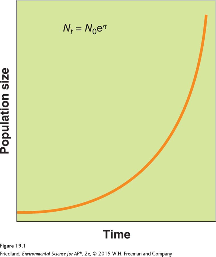
When populations are not limited by resources, growth can be very rapid because more births occur with each step in time. When graphed, the exponential growth model produces a J-
One way to think about exponential growth in a population is to compare it to the growth of a bank account where N0 is the account balance and r is the interest rate. Let’s say you put $1,000 in a bank account at an annual interest rate of 5 percent. After 1 year the new balance in the account would be:
Nt = $1,000 ×e(0.05×1)
Nt = $1,051.27
In the second year, the balance in the account would be:
Nt = $1,000 × e(0.05×2)
Nt = $1,105.17
In the tenth year, the account would grow to a balance of $1,648.72. Moving forward to the twentieth year, the same 5 percent interest rate would produce a balance of $2,718.28.
198
Applying an annual rate of growth to an increasing amount, whether money in a bank account or a population of organisms, produces rapid growth over time. Exponential growth is density independent because the value will grow by the same percentage every year. “Do the Math: Calculating Exponential Growth” gives a step-
The exponential growth model is an excellent starting point for understanding population growth. Indeed, there is solid evidence that real populations—
The logistic growth model describes populations that experience a carrying capacity
Logistic growth model A growth model that describes a population whose growth is initially exponential, but slows as the population approaches the carrying capacity of the environment.
S-
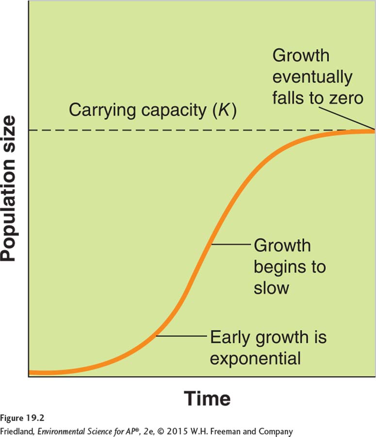
While the exponential growth model describes a continuously increasing population that grows at a fixed rate, populations do not experience exponential growth indefinitely. For this reason, ecologists have modified the exponential growth model to incorporate environmental limits on population growth, including limiting resources. The logistic growth model describes a population whose growth is initially exponential, but slows as the population approaches the carrying capacity of the environment (K). As we can see in FIGURE 19.2, if a population starts out small, its growth can be very rapid. As the population size nears about one-
The logistic growth model is used to predict the growth of populations that are subject to density-
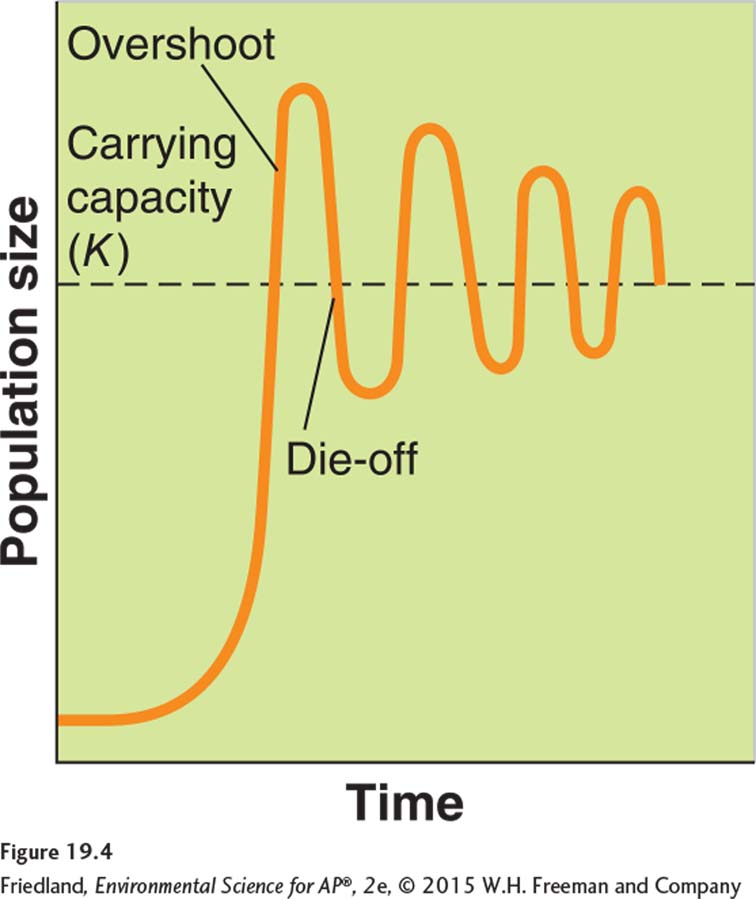
Overshoot When a population becomes larger than the environment’s carrying capacity.
Die-
One of the assumptions of the logistic growth model is that the number of offspring produced depends on the current population size and the carrying capacity of the environment. However, many species of mammals mate during the fall or winter, and the number of offspring that develop depends on the food supply at the time of mating. Because these offspring are not actually born until the following spring, there is a risk that food availability will not match the new population size. If there is less food available in the spring than needed to feed the offspring, the population will experience an overshoot by becoming larger than the environment’s carrying capacity. As a result of this overshoot, there will not be enough food for all the individuals in the population, and the population will experience a die-
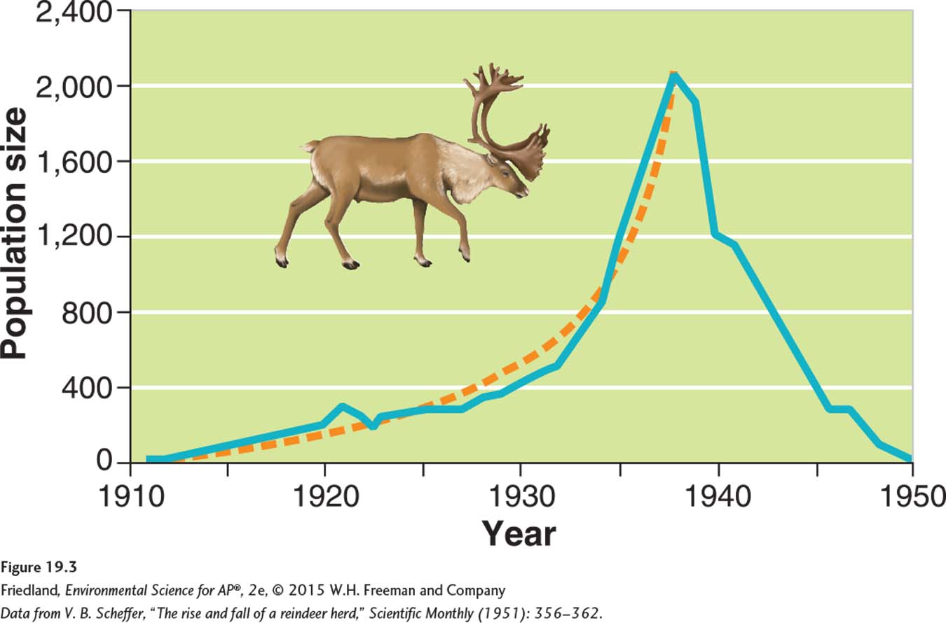
The reindeer (Rangifer tarandus) population on St. Paul Island in Alaska is a good example of this pattern. As you can see in FIGURE 19.3, a small population of 25 reindeer that was introduced to the island in 1910 grew exponentially until it reached more than 2,000 individuals in 1938. After 1938, the population crashed to only 8 animals, most likely because the reindeer ran out of food.
199
Such die-
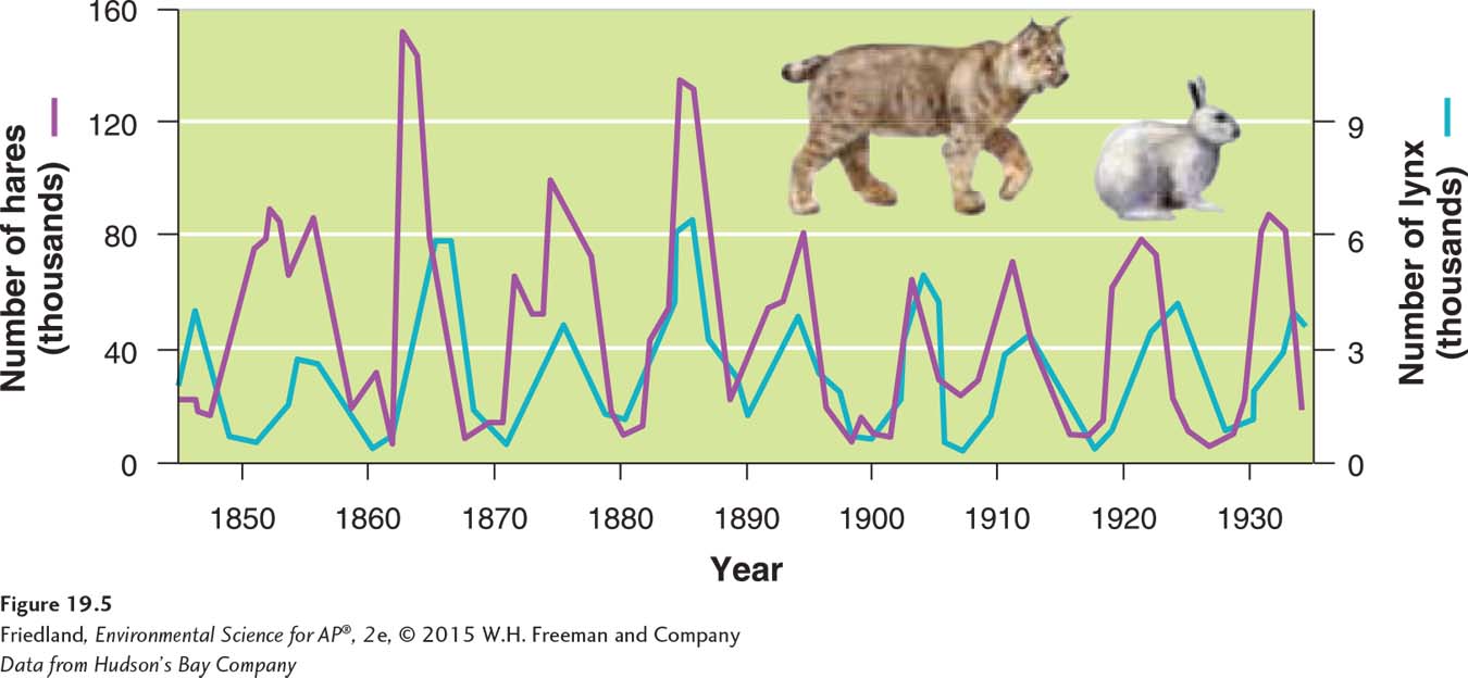
So far we have considered only how populations are limited by resources such as food, water, and the availability of nest sites. Predation may play an important additional role in limiting population growth. A classic example is the relationship between snowshoe hares (Lepus americanus) and lynx (Lynx canadensis) that prey on them in North America. Trapping records from the Hudson’s Bay Company, which purchased hare and lynx pelts for nearly 90 years in Canada, indicate that the populations of both species cycle over time. FIGURE 19.5 shows how this interaction works. The lynx population peaks 1 or 2 years after the hare population peaks. As the hare population increases, it provides more prey for the lynx, and thus the lynx population begins to grow. As the hare population reaches a peak, food for hares becomes scarce, and the hare population dies off. The decline in hares leads to a subsequent decline in the lynx population. Because the low lynx numbers reduce predation, the hare population increases again.
200
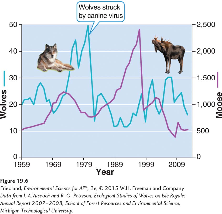
A similar case of predator control of prey populations has been observed on Isle Royale, Michigan, an island in Lake Superior. Wolves (Canis lupus) and moose (Alces alces) have coexisted on Isle Royale for several decades. Starting in 1981, the wolf population declined sharply, probably as a result of a deadly canine virus. As wolf predation on moose declined, the moose population grew rapidly until it ran out of food and experienced a large die-
Species have different reproductive strategies and distinct survivorship curves
Population size most commonly increases through reproduction. Population ecologists have identified a range of reproductive strategies in nature.
K-selected Species
K-selected species A species with a low intrinsic growth rate that causes the population to increase slowly until it reaches carrying capacity.
K-selected species are species that have a low intrinsic growth rate that causes the population to increase slowly until it reaches the carrying capacity of the environment. As a result, the abundance of K-selected species is determined by the carrying capacity, and their population fluctuations are small. The name “K-selected species” refers to the fact that these populations commonly exist close to their carrying capacity, denoted as K in population models.
201
K-
r-selected Species
r-selected species A species that has a high intrinsic growth rate, which often leads to population overshoots and die-
At the opposite end of the spectrum from K-selected species, r-selected species have a high intrinsic growth rate that often leads to population overshoots and die-
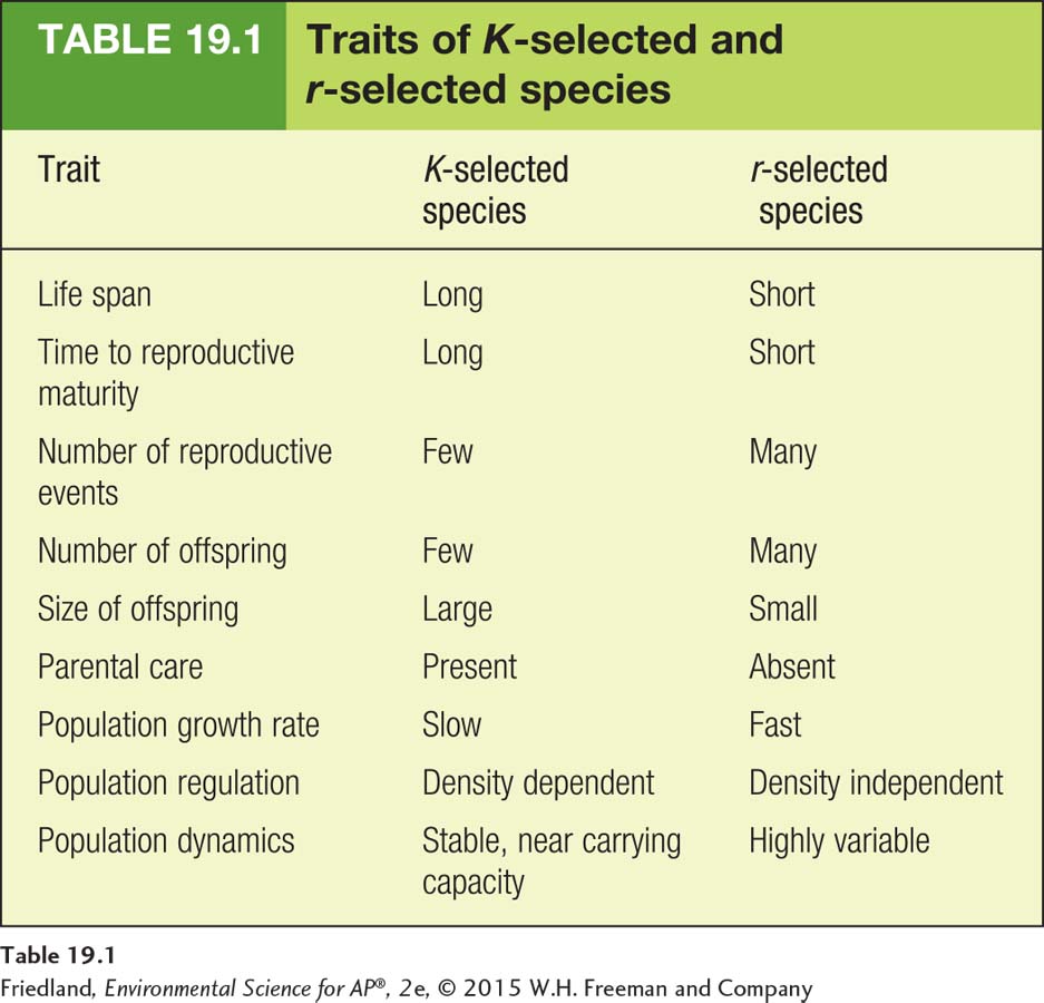
TABLE 19.1 summarizes the traits of K-selected and r-selected species. These two categories represent opposite ends of a wide spectrum of reproductive strategies. Most species fall somewhere in between these two extremes, and many exhibit combinations of traits from the two extremes. For example, tuna and redwood trees are both long-
Survivorship curve A graph that represents the distinct patterns of species survival as a function of age.
Type I survivorship curve A pattern of survival over time in which there is high survival throughout most of the life span, but then individuals start to die in large numbers as they approach old age.
Type II survivorship curve A pattern of survival over time in which there is a relatively constant decline in survivorship throughout most of the life span.
Type III survivorship curve A pattern of survival over time in which there is low survivorship early in life with few individuals reaching adulthood.
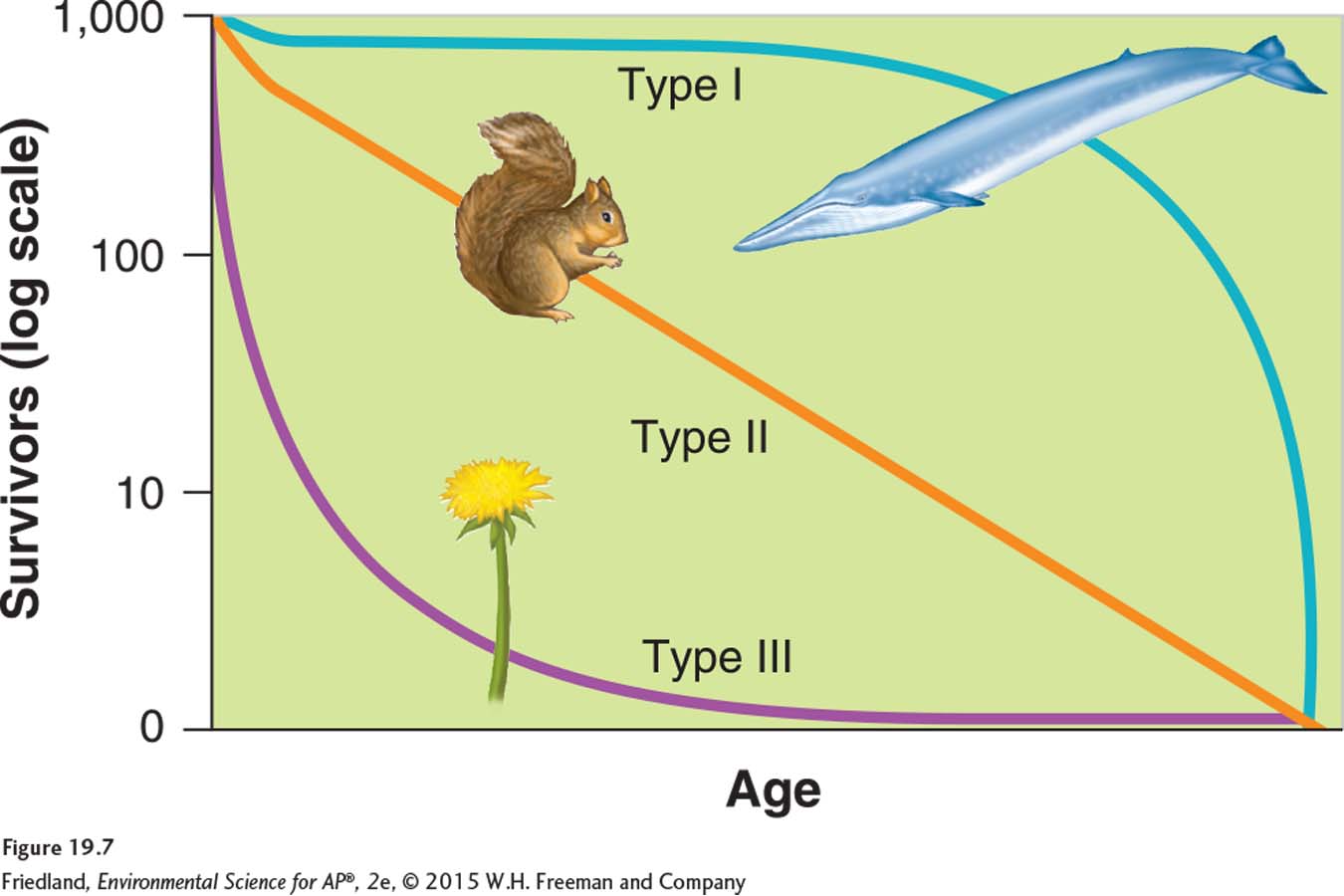
In addition to different reproductive strategies, species have distinct patterns of survival over the life span of individuals. These patterns can be plotted on a graph as survivorship curves, as shown in FIGURE 19.7. There are three basic types of survivorship curves. A type I survivorship curve has high survival throughout most of the life span, but then individuals start to die in large numbers as they approach old age. Species with type I curves include K-selected species such as elephants, whales, and humans. In contrast, a type II survivorship curve has a relatively constant decline in survivorship throughout most of the life span. Species with a type II curve include corals and squirrels. A type III survivorship curve has low survivorship early in life with few individuals reaching adulthood. Species with type III curves include r-selected species such as mosquitoes and dandelions.
202
Interconnected populations form metapopulations
Cougars (Puma concolor)—also called mountain lions or pumas—
Corridor Strips of natural habitat that connect populations.
Metapopulation A group of spatially distinct populations that are connected by occasional movements of individuals between them.
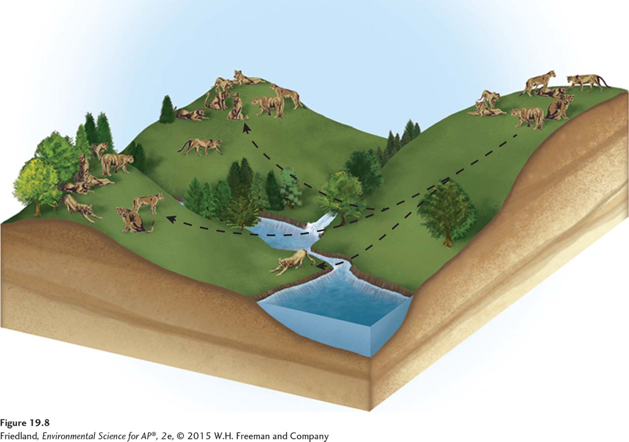
Because areas of desert separate the cougar’s mountain habitats, we can consider the cougars of each mountain range to be a distinct population. Each population has its own dynamics based on local abiotic conditions and prey availability: Large mountain ranges support large cougar populations and smaller mountain ranges support smaller cougar populations. As FIGURE 19.8 shows, cougars sometimes move between mountain ranges, often using strips of natural habitat that connect the separated populations. Strips of natural habitat that connect populations are known as corridors and provide some connectedness among the populations. A group of spatially distinct populations that are connected by occasional movements of individuals between them is called a metapopulation.
Inbreeding depression When individuals with similar genotypes—
The connectedness among the populations within a metapopulation is an important part of each population’s overall persistence. Small populations are more likely than large ones to go extinct. As we have seen, small populations contain relatively little genetic variation and therefore may not be able to adapt to changing environmental conditions. Small populations can also experience inbreeding depression. Inbreeding depression occurs when individuals with similar genotypes—
Small populations are also more vulnerable than large populations to catastrophes such as particularly harsh winters that drive down their populations to critically low numbers. In a metapopulation, occasional immigrants from larger nearby populations can add to the size of a small population and introduce new genetic diversity, both of which help reduce the risk of extinction.
Metapopulations can also provide a species with some protection against threats such as diseases. A disease could cause a population living in a single large habitat patch to go extinct. But if a population living in an isolated habitat patch is part of a much larger metapopulation, then, while a disease could wipe out that isolated population, immigrants from other populations could later recolonize the patch and help the species to persist.
Because many habitats are naturally patchy across the landscape, many species are part of metapopulations. For instance, numerous species of butterflies specialize on plants with patchy distributions. Some amphibians live in isolated wetlands, but occasionally disperse to other wetlands. The number of species that exist as metapopulations is growing because human activities have fragmented habitats, dividing single large populations into several smaller populations. Identifying and managing metapopulations is thus an increasingly important part of protecting biodiversity.