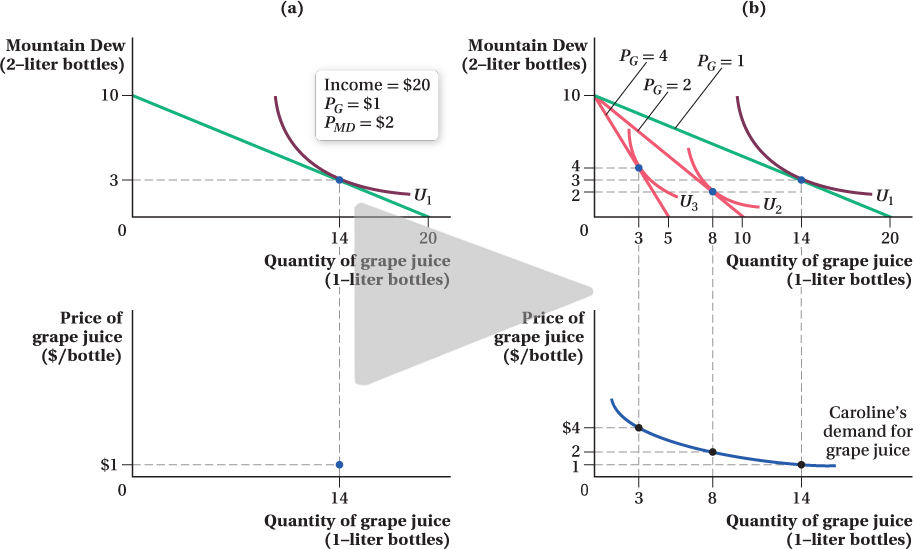
Figure 5.7 Building an Individual’s Demand Curve
(a) At her optimal consumption bundle, Caroline purchases 14 bottles of grape juice when the price per bottle is $1 and her income is $20. The bottom panel plots this point on her demand curve, with the price of grape juice on the y-axis and the quantity of grape juice on the x-axis.(b) A completed demand curve consists of many of these quantity-price points. Here, the optimal quantity of grape juice consumed is plotted for the prices $1, $2, and $4 per bottle. This creates Caroline’s demand curve, as shown in the bottom panel.