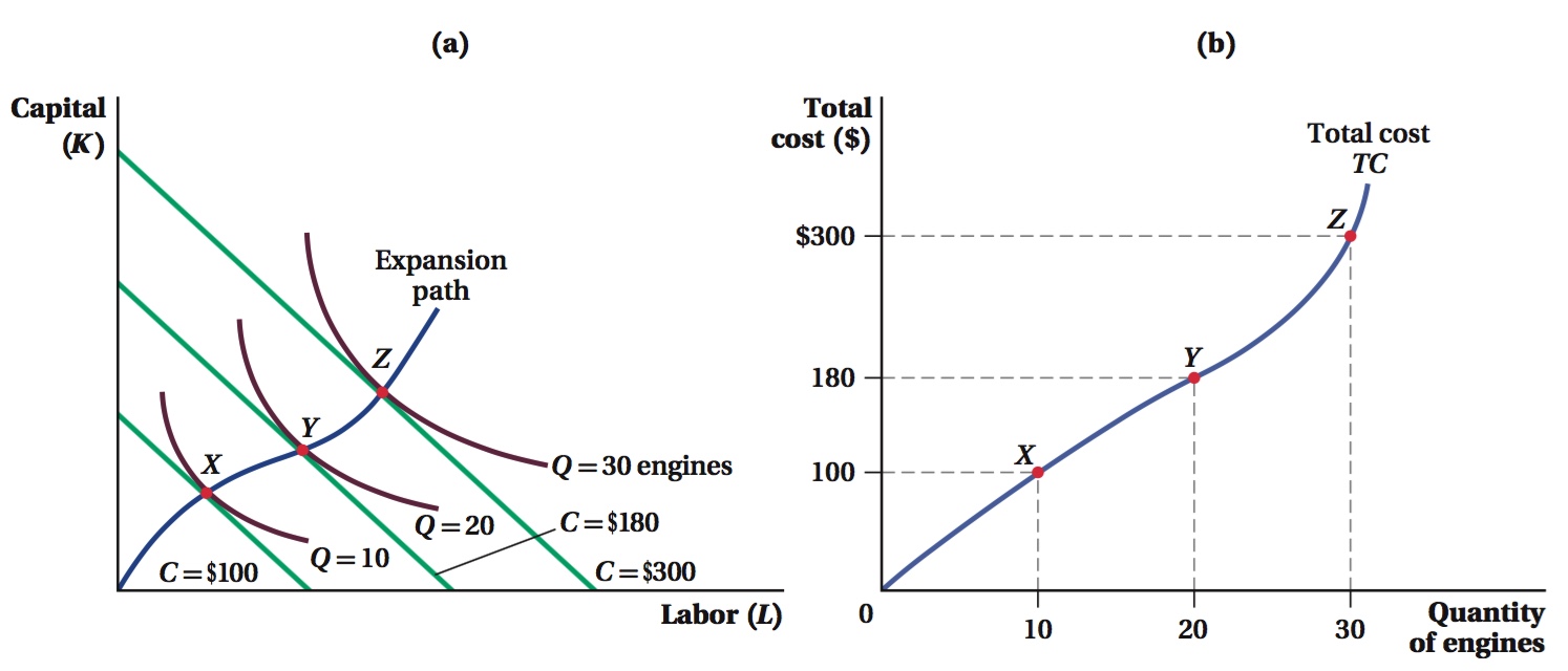
Figure 6.15 The Expansion Path and the Total Cost Curve
(a) The expansion path for Ivor’s Engines MAPs the optimal input combinations for each quantity Q. Here, points X, Y, and Z are the cost-minimizing input combinations given output levels Q = 10, Q = 20, and Q = 30, respectively.(b) The total cost curve for Ivor’s Engines is constructed using the isocost lines from the expansion path in panel a. The cost-minimizing input combinations cost $100, $180, and $300 at output levels Q = 10, Q = 20, and Q = 30, respectively.