Block Pricing
The practice of reducing the price of a good when the customer buys more of it.
We call the strategy in which a firm reduces the price of a good if the customer buys more of it block pricing. You see this sort of thing all the time. Buying a single 12-ounce can of Pepsi might cost $1, but a six-pack of 12-ounce cans costs only $2.99. However, unlike indirect price discrimination (such as quantity discounts), block pricing does not require that buyers have different demand curves and price sensitivities. All buyers of Pepsi may, in fact, have the same demand curve, but Pepsi could still gain producer surplus from providing buyers with an option to buy a larger quantity of soda at a lower price.
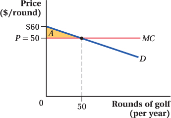
Consider Figure 10.8, which shows a demand curve for Walmart’s photo holiday cards. Here, we assume this is the demand curve of just one customer (or we could suppose all customers have this same demand curve), so the firm is not trying to price-discriminate across customers with different types of demand, as would be the case if Walmart offers quantity discounts. If Walmart follows the pricing rule for firms with market power in Chapter 9, it will pick the quantity at which marginal revenue equals marginal cost and charge a price equal to the height of the demand curve at that quantity. In the figure, the monopoly quantity is 100 cards and the price is 25 cents per card. Walmart’s producer surplus from pricing at that point equals the area of rectangle A.
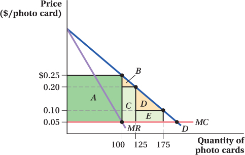
Figure 10.8: Figure 10.8 Block Pricing
Figure 10.8: D is the demand curve of an individual consumer of Walmart’s photo cards. Under monopoly pricing, Walmart sells at the point on the demand curve corresponding to the quantity where MR = MC (Q* = 100 photo cards, P* = $0.25 per card). When Walmart can prevent resale, it can use a block pricing strategy instead. It could still sell the first 100 at a price of $0.25 per card, while charging a lower price of $0.20 each for the next 25 photos purchased (for a total quantity of 125 cards) and $0.10 each for the next 50 cards (for a total of 175 cards). Producer surplus increases from area A to A + C to A + C + E, respectively, and consumer surplus increases by area B and areas B + D, respectively.
If Walmart can prevent resale, however, it doesn’t have to charge a single price. Suppose it offers the first 100 holiday cards for sale at 25 cents each, but then allows a consumer to buy as many as 25 more cards (numbers 101 to 125) at a lower per-unit price of 20 cents each. The customer will take advantage of this offer because the incremental purchase at the lower price yields an additional consumer surplus equal to the area of triangle B. Walmart is better off, too, because it adds an additional amount of producer surplus equal to the area of rectangle C.
∂ The online appendix finds profit-maximizing block prices.
Walmart could keep offering discounted prices on larger quantities. For example, it could offer the next 50 cards, up to the 175th photo card, for 10 cents each. Again, the consumer will take the deal because the consumer surplus from that block of cards (area D in the figure) is positive. Walmart also comes out ahead because it earns producer surplus E. Note that the price strategy we just described could also be expressed in the following way: 100 units are $25, 125 units are $30, and 175 units are $35. Even if all customers have this same demand, all will opt to purchase 175 cards at a price of $35 and Walmart still increases its producer surplus. (This is why block pricing is different from the quantity discounts we saw when discussing indirect price discrimination. Here, no customer sorting needs to occur for Walmart to gain producer surplus.)
A block-pricing strategy like this raises more producer surplus for a firm than does the conventional single-price monopoly strategy because it allows a firm to better match the prices of different quantities of its output to consumers’ valuations of those quantities. For the first set of units that customers buy—the units for which customers have a high willingness to pay—the firm charges a relatively high price. With block pricing, the firm doesn’t have to completely give up selling a large number of units by charging that initial high price. Block pricing lets it sell additional units of its product, those for which consumers have lower willingness to pay, at lower prices.
This example shows how block pricing can work for even a single customer type, though if there were lots of identical customers, the firm would need to be able to prevent resale to avoid being undercut by its own customers.
Two-Part Tariffs
A pricing strategy in which the payment has two components, a per-unit price and a fixed fee.
Another pricing strategy available to firms with market power and identical consumers is the two-part tariff, a pricing strategy in which a firm breaks the payments for a product into two parts. One component is a standard per-unit price. The second is a fixed fee that must be paid to buy any amount of the product at all, no matter how large or how small.
For example, a lot of mobile phone “unlimited service” calling plans have this structure. You might pay, say, $70 a month for service and then be able to talk, text, and stream as much as you would like at no additional cost. Here, the fixed fee portion of the two-part tariff is $70 and the per-unit price is zero (though for other markets and products, the per-unit price is often positive). A video game system such as Microsoft’s Xbox is like a two-part tariff, too. The cost of the console itself is the fixed fee and the cost of the individual games represents the per-unit price.
To see the advantage of using a two-part tariff for a firm with market power, consider the market in Figure 10.9. It shows the demand for mobile phone service offered by the firm, the marginal revenue curve corresponding to demand, and the firm’s constant marginal cost.
Figure 10.9: Figure 10.9 Two-Part Tariff
Figure 10.9: As a single-price monopoly, a mobile phone service will sell 3 GB of mobile service per month at a price of $20 per GB. Using a two-part tariff, however, the firm can increase its producer surplus from rectangle B to the triangle A + B + C. To do this, it will charge the per-unit price of $10 per GB, where D = MC, and set a fixed fee equal to the consumer’s surplus at this quantity, the area A + B + C. Under this pricing scheme, the firm will sell 6 GB of mobile service per month.
The firm’s conventional single-price monopoly profit-maximizing quantity is found where marginal revenue equals marginal cost. The quantity at which this condition holds is 3 GB per month, and the price at which consumers are willing to purchase that quantity is $20 per GB. At the price of $20 per GB, the consumer surplus is area A and the firm’s producer surplus is rectangle B.
Now suppose instead that the firm uses the following two-part tariff pricing structure. First, it reduces the per-unit price all the way to marginal cost, $10 per GB. This change increases the number of units it sells from 3 GB to 6 GB, but drives per-unit profit to zero. However, the firm knows that each customer will buy a quantity of 6 GB per month at this price and have a consumer surplus equal to area A + B + C as a result. Knowing that this consumer surplus represents the willingness of the consumers to pay above the market price, the firm will set a fixed fee to try to capture that consumer surplus. Therefore, the firm decides to set the fixed-fee portion of the two-part tariff equal to A + B + C. This fee is not per GB; it’s a one-time-per-month fee for any consumer who wants to buy any number of units at $10 per GB.
What happens under this two-part tariff pricing structure? At a unit price of $10 per GB, the consumer buys 6 GB. This part of the price structure doesn’t make the phone company any money, because its marginal cost of delivering service is also $10 per GB. However, the company is also charging the fixed fee A + B + C. And importantly, the consumer is willing to pay that, because if she uses 6 GB, she will enjoy consumer surplus equal to the same area. The company has set the size of the fixed fee so that the consumer is no worse off (and actually it could make her strictly better off if it charged just a touch less than A + B + C) than if she bought nothing. By using a two-part tariff, the firm captures the entire surplus in the market for itself, as opposed to only area B under standard market power pricing.
Again, if you apply this insight to a market with many identical customers, the ability to prevent resale would be crucial for making the pricing strategy work. If the phone company couldn’t prevent resale, one customer could pay the fixed fee, buy up a huge amount of GB at marginal cost, sell off these extra GB at a small markup to other consumers who did not pay the fixed fee, and make lots of money. For example, if the consumer could rig her phone so other people would pay her $6 per GB to stream off it when she wasn’t using the phone, this would defeat the company’s strategy.
 See the problem worked out using calculus
figure it out 10.5
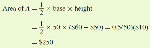
You have been hired as an intern at the Golden Eagle Country Club Golf Course. You have been assigned the task of creating the pricing scheme for the golf course, which typically charges an annual membership fee and a per-use cost to its customers. Each of your customers is estimated to have the following demand curve for rounds of golf per year:
If Golden Eagle can provide rounds of golf at a constant marginal cost of $50 and charges that amount per round of golf, what is the most that members would be willing to pay for the annual membership fee?
This pricing scheme, with an annual membership fee and a per-unit price, is a two-part tariff. If the price per round of golf is set at P = $50, then each member will want to play
With this knowledge, we can determine the maximum annual membership fee each customer is willing to pay. This will be equal to the amount of consumer surplus the customer will get from playing 50 rounds of golf each year at a price of $50 per round.
To calculate consumer surplus, it is easiest to draw a diagram, plot the demand curve, and find the area of consumer surplus. To simplify matters, let’s rearrange the demand function into an inverse demand function:
The vertical intercept is 60 and the consumer surplus is the area below the demand curve and above the price of $50, area A. We can calculate the area of triangle A:
If the golf course set the price of a round of golf at $50, the consumer would purchase 50 rounds per year. This gives the golfer a consumer surplus equal to $250. Therefore, customers would be willing to pay up to $250 for an annual membership.
Being able to capture the entire surplus in the market is great if you’re running a firm, but it’s important to realize that a firm can attain this extreme result only if its customers have the same demand curve. The problem is much more complicated when there are customers with different demand curves.
For this more advanced two-part tariff pricing case, think about a firm that faces two kinds of customers whose demand curves for the firm’s product are shown in Figure 10.10. Panel a shows the demand curve of the firm’s relatively low-demand customers, while panel b shows the demand of the firm’s relatively high-demand customers. If the firm tries to use a two-part tariff where it sets the unit price at marginal cost MC and the fixed fee at A + B + C, it will capture all of the surplus from the relatively low-demand customers in panel a but leave a lot of surplus to the relatively high-demand customers in panel b, because area A + B + C is much smaller than area D + E + F. If the firm instead sets the fee at D + E + F to capture the surplus of the high-demand customers, low-demand customers won’t buy at all. This is not necessarily better than the first strategy. If the firm has a lot of low-demand customers, this could represent a big loss for the firm, even if the reduction in profit from losing any given low-demand customer might be small. So, neither approach is perfect. Computing the profit-maximizing two-part tariff when consumers have different demands is a mathematical challenge beyond the scope of this book, but it usually entails a unit price above the firm’s marginal cost.
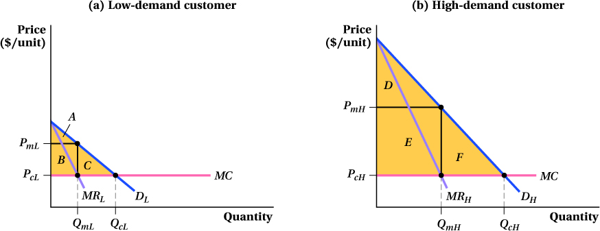
Figure 10.10: Figure 10.10 Two-Part Tariff with Different Customer Demands
Figure 10.10: (a) For low-demand customers, the firm would want to sell a quantity of QcL, charge a per-unit price of PcL and a fixed fee equal to the consumer surplus A + B + C. Because this is much lower than the consumer surplus for high-demand customers (D + E + F in panel b), such a pricing strategy will leave a lot of surplus to the high-demand customers in the market.
(b) For high-demand customers, the firm would want to sell a quantity of QcH, and charge a per-unit price of PcH and a fixed fee equal to D + E + F. Because this fixed fee is higher than the consumer surplus for low-demand customers, low-demand customers won’t buy anything.