528

We’ve restricted our attention so far to perfectly competitive factor markets. Individual demanders of factors—firms—choose how much of the factors to buy while taking their price as given, an equilibrium price that is determined in the factor markets by the forces of supply and demand. Suppliers of factors do the same: They take their price as given and decide what quantity to supply at that price.

As we have learned in earlier chapters, perfectly competitive markets are rare in the real world. In the next sections, we look at what happens when factor demanders or suppliers are not price takers. We begin by looking at cases in which buyers have market power.

We are already familiar from Chapter 9, Chapter 10 and Chapter 11 with how markets work when sellers have some monopoly power—that is, when they recognize their decision about how much to sell affects the price at which their products will be sold. There is a buyer-side analogy to monopoly that is important in some factor markets. When a buyer recognizes that its choice of how much to buy affects the market price of what it purchases, this is a type of market power called monopsony power.

There are many examples of concentrated buyers who are likely to have some monopsony power. Pepsi and Coca-Cola, Target and Walmart, Apple and Samsung—each of these companies is so large that it cannot only influence the prices buyers will pay for its output, but also can influence the prices each pays to its factor suppliers. Nabisco dominates the market for fig-based snacks with its Fig Newtons cookies and it buys figs from a large number of fig growers (the factor suppliers). If Nabisco decides to make fewer Fig Newtons, this will influence the price of figs.

To make things more concrete, let’s think about the market for oil workers in the Athabasca Oil Sands (AOS), which are located in a remote area of northern Alberta, Canada. If you live and work in this region, it’s likely you work in oil production and have limited ability to change jobs unless you leave the area. At the same time, only a few large companies account for most of the oil production and employment there.

These facts imply that employers in the AOS region have some monopsony power. Because each company accounts for a considerable share of the total market demand for labor, the more labor it hires, the higher the wage will rise. Note that just as we discussed regarding the relationship between monopoly and market power, a firm can have monopsony power without being literally the only buyer. The key is that it is not a price (wage) taker when it buys (hires).

We know from our analysis earlier in this chapter that in a competitive factor market, oil companies would hire workers until the marginal revenue product of those oil workers equaled the market wage. That wage would be set by market-level supply and demand, and firms would take it as given. However, a monopsonist like Syncrude (one of the biggest oil companies operating in Alberta) is a buyer with market power. Because its hiring is such a large part of market labor demand, it influences the wage. In other words, it faces an upward-sloping (not horizontal) labor supply curve. The more people Syncrude hires, the higher the wage it has to pay. As a result, a monopsonist like Syncrude faces a dilemma that is similar to that dealt with by a monopolist.

We can think about Syncrude’s decision in terms of marginal expenditure, ME, the incremental expenditure from buying one more unit of labor. Buyers with no market power—the kind we have been dealing with in this chapter until now—can buy as many units as they want without affecting the price. Their marginal expenditure is just the market price (the wage, in labor markets) irrespective of the quantity they buy. This isn’t so for monopsonists, however. If Syncrude wants to hire more labor, the increase in quantity demanded is large enough to require the market wage to rise to bring the additional labor into the market. This means Syncrude’s marginal expenditure (ME) when it buys an incremental unit of labor isn’t just the higher wage for that one worker. It is that wage plus the incremental wage increase it has to pay to all its other non-incremental workers.

529

This is easier to understand in an example. Suppose hiring 1,000 employees would cost Syncrude a wage of $50,000 per employee, while hiring 1,100 employees would raise the wage to $60,000 per employee (here, we’re treating the marginal unit of labor as being 100 employees). Syncrude’s total payroll for employing 1,000 workers would then be $50 million (1,000 × $50,000), while its payroll for hiring 1,100 workers would be $66 million (1,100 × $60,000). Therefore, its marginal expenditure (ME) for one incremental unit of labor (100 employees) is not just the $6 million it pays to hire 100 extra workers ($60,000 × 100) but $16 million ($66 million for 1,100 workers – $50 million for 1,000 workers). Syncrude’s extra hiring requires the company to pay an extra $10 million ($10,000 to each of its 1,000 non-incremental workers) beyond the $6 million it has to pay the extra hires. Therefore, just as marginal revenue differs from the price for a monopoly supplier, marginal expenditure differs from the price (wage) for a monopsony buyer. The direction of the difference is opposite, though: While marginal revenue is always less than the price for a monopolist, marginal expenditure is always more than the price for a monopsonist.

We can mathematically express marginal expenditure for a monopsonist as the price plus the amount that prices would change from increasing quantity times the quantity:

ME = P + (ΔP/ΔQ) × Q

If this looks familiar, it is because it’s very much like the definition of marginal revenue from Chapter 9. The difference is that for monopoly power and marginal revenue, ΔP/ΔQ is negative because it depends on the downward-sloping demand curve. Here, for monopsony power and marginal expenditure, ΔP/ΔQ is positive because it is tied to the upward-sloping supply curve. Notice that for a buyer who faces a flat supply curve—that is, a buyer who has no monopsony power and therefore takes the factor’s purchase price as given—ΔP/ΔQ is zero and ME = P, as we saw earlier.

When Syncrude hires labor as a monopsonist, it faces an upward-sloping supply curve of labor. This means Syncrude’s ME on labor is always greater than the wage, and Syncrude’s labor ME curve will always be above the labor supply curve it faces, as shown in Figure 13.11. For a linear supply curve like S, as depicted in the figure, the ME curve will be twice as steep as the supply curve, just like marginal revenue is for the demand curve (see Chapter 9).

We saw earlier in the chapter that price-taking buyers purchase a factor until its marginal revenue product equals its price (which equals the input’s price). This means we can express the optimal amount of inputs for a price-taking buyer as the quantity that equates the marginal revenue product to the marginal expenditure: MRP = ME. This same expression holds true for a monopsonist like Syncrude as well as for a competitive firm. It’s just a matter of defining ME. If a monopsonist buys more of an input than the MRP = ME amount, then the additional amount the monopsonist spends to buy those inputs will exceed the revenues it earns from them. If the firm buys fewer inputs than the MRP = ME quantity, then by buying more of the input, it could raise revenues by a greater amount than its expenditures on the inputs. Only when MRP = ME is the monopsonist buying the profit-maximizing amount of inputs.

530

While the competitive and monopsony cases have the same MRP = ME rule for input demand, ME is different for a monopsonist than for a price-taking buyer. We know that ME = P for a price taker, while for a monopsonist, ME = P + (ΔP/ΔQ) × Q, which is always greater than P. Therefore for the same MRP and input supply curves, a monopsonist will buy fewer inputs than a price-taking firm, because a monopsonist’s marginal expenditure on a factor will equal its marginal revenue product at a lower quantity of the factor. Because Syncrude knows it drives up the wage by hiring more workers, it holds back a little. Hiring an incremental unit of input is more expensive for it than for a price-taking firm. In this way, a monopsonist restricts purchases just as a monopolist restricts sales.

531

To find the equilibrium of a market when a buyer has monopsony power, we follow the same three-step procedure that we did in the monopoly power case, but looking at the supply curve rather than the demand side. Specifically:

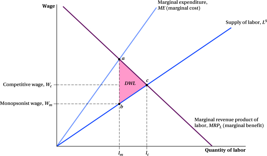
Figure 13.11 shows this analysis for Syncrude. Syncrude’s marginal revenue product curve for labor is MRP_L, and the labor supply curve it faces is S. We first plot the marginal expenditure curve, ME, that corresponds to the supply curve. It is, as we know, above S, and because S is linear, it is twice as steep. Second, we find the optimal quantity of labor for Syncrude to hire by identifying where the ME curve intersects MRP_L. This intersection is at point a in the figure and the quantity is l_m. Third, we find the wage Syncrude pays by reading off the level of the supply curve at quantity l_m. This is point b, and the corresponding wage W_m is what Syncrude has to pay workers to make them willing to supply Syncrude with its desired quantity of labor l_m.

The monopsony quantity l_m and wage W_m are different than those that would be found if Syncrude’s labor demand (embodied in MRP_L) was instead the demand of a set of perfectly competitive buyers. In that case, the equilibrium wage and quantity of labor would be identified by point c, the intersection of the market demand and supply curves—quantity l_c and wage W_c. Monopsony results in a smaller quantity of the input hired and at a lower price than would be found in a competitive market.

Just as with monopoly power, monopsony creates a deadweight loss, DWL. This arises because there will be some workers who would work for wages less than the marginal revenue product they create for the firm, but they aren’t hired because it would raise overall wages too much. In the Syncrude case shown in Figure 13.11, the units of labor that have social value but are not sold are those between l_m and l_c. The total size of the deadweight loss from this unsold labor is the total surplus they would have created had they been sold. Any given unit of labor has a surplus equal to the vertical distance between the labor demand curve (the value of the labor to Syncrude) and the labor supply curve (which shows what workers must be paid to be willing to work). If we add up the surplus of all the labor that is unsold in the monopsony market but would be sold in the competitive market, this is the triangular area labeled DWL in the figure. This triangle is the deadweight loss of monopsony power.

532