We now understand how to analyze investment choices using net present value analysis, and we have developed a sense of how the interest rate used in NPV analysis is determined. There is one important component of these decisions we’ve ignored until now: risk. What if things don’t work out as we expect them to? In real life, firms and consumers face a lot of uncertainty when making investment decisions. Sometimes investments flop. In this section, we discuss the ways to analyze NPVs while taking uncertainty into account, including situations in which investors have the option of waiting to gather more information before deciding to invest.

The basic way to incorporate risk into NPV investment analysis is to compute NPV as an expected value, that is, by weighting each payoff by the probability that it happens. Any risky payout can be described as a combination of two things: the different payouts that could possibly happen, and the probability of each possible outcome occurring.

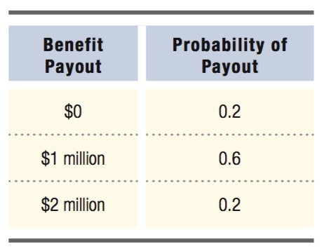
Consider an example of a risky investment that will pay an uncertain benefit in one year. Table 14.4 shows the possible benefits along with the probabilities of their occurrence. Looking at these possible outcomes, we see that the investment could perform poorly and earn no return with a small probability (0.2, or 20%), do very well and deliver a $2 million payout with a small probability (0.2), or, most likely, yield a modest $1 million payout with higher probability (0.6).6

We use the concept of expected value to evaluate the situation. The expected value of any uncertain outcome is the sum of the product of each possible outcome/payment and the probability of that outcome/payment. (Equivalently, it is the probability-weighted average outcome.) In general terms, for an uncertain outcome with N possible payments,

Expected value = (p₁ × M₁) + (p₂ × M₂) + . . . + (p_N × M_N)

where p₁, p₂, . . . p_N are, respectively, the probabilities of payments 1, 2, and so on, and M₁, M₂, . . . M_N are the payments themselves. So, in our example investment above, the expected benefit payout is

Expected benefit payout = (0.2 × $0) + (0.6 × $1 million) + (0.2 × $2 million)

= $0 + $0.6 million + $0.4 million

= $1 million

For payment flows that are guaranteed—that is, for which there is no uncertainty—computing expected value is easy. Because the payment is certain, its probability is 1 (or 100% if you prefer). Therefore, the expected value is just 1 times the guaranteed payment. An investment with a $1 million guaranteed payout has an expected payout value of $1 million.

556

Using expected value, then, all of the NPV calculations hold up exactly the same way as before, but you just need to multiply outcomes by their probabilities.

Evaluating an investment using expected value provides a natural way to incorporate risk into the NPV calculation. One way risk can influence decisions is by creating an incentive to postpone investments and gather more information. This incentive, known as the option value of waiting, arises if waiting will resolve some of the uncertainty about the investment before deciding whether to go forward with the investment. (The name refers to the fact that an investor’s option to postpone an investment decision is conceptually related to financial options—contracts that give someone the right, but not the obligation, to buy or sell an item.)

Let’s use an example to see how this operates. It’s 2016 and you want to get a new, high-tech television. There is an emerging battle over advanced television formats between 4K televisions and HD 3D televisions. Your next TV can be a 4K TV or a mythical Hyper-3D HD system, but you don’t have enough money or space to be able to buy both. It’s not clear what the future of TV broadcasting will be; maybe channels will eventually be broadcast in 4K, or maybe they’ll decide to go with Hyper-3D instead. This is what economists call a “standards war”: It’s likely only one format will succeed in becoming the standard technological platform in the market. The other will probably die off. Suppose the battle is expected to be settled one year later. Therefore, if you buy the wrong television, within a year, you won’t be able to see your favorite shows using it. If you choose correctly, everything will be fine.

Let’s apply some numbers to see how this uncertainty affects the NPV and the option value of buying a television. Suppose the interest rate is 5%, 4K TVs cost $1,350, and HD 3D TVs cost $1,200. Furthermore, each type of television gives its owner $150 per year of value forever if his or her favorite shows are broadcast in that format and $0 if not (i.e., if the TV’s format has lost the standards war).

Given this information, the value of a 4K television in the first year is –$1,350 + $150 = –$1,200. For every year following that, a 4K TV offers a $150 benefit if that is the format that channels are broadcast in. Using the formula we discussed above, the total PDV of this infinite stream of $150 benefits is $150/0.05 = $3,000. The Hyper-3D television has a first-year value of –$1,200 + $150 = –$1,050 and a per-year $150 benefit after that, if the Hyper-3D format becomes the standard. In this case, the PDV of the Hyper-3D’s infinite stream of $150 benefits is also $3,000.

Finally, suppose analysts believe that 4K has a 75% chance of winning the standards war and Hyper-3D has a 25% chance.

Now we have everything we need to compute the net present value (NPV) of buying each television in 2016. If you purchase a 4K TV, the first year’s payouts include the price you pay for the television ($1,350) and the $150 benefit you receive from it for that year. After that, starting in 2017, there is a 75% chance 4K will win the standards war and you will receive a $150 annual benefit forever (PDV = $3,000). On the other hand, there is a 25% chance Hyper-3D will win the standards war and your 4K TV will become worthless. Therefore, the NPV of buying the 4K in 2016 is

4K NPV₂₀₁₆ = (–$1,350 + $150) + 0.75 × ($3,000/1.05) + 0.25 × ($0/1.05)

= –$1,200 + 0.75 × $2,857.14 + 0.25 × $0

= –$1,200 + $2,142.86 + $0 = $942.86

557

Notice that this NPV calculation is an expected value—we’ve weighted each cost and benefit by the probability that it occurs. The payments in the first year, the $1,350 outlay to buy the television and the $150 benefit you receive from it, are guaranteed, so they are multiplied by 1. For future payouts, we multiply the $3,000 PDV benefit stream received if 4K TV wins the standards war by the 75% probability that 4K does, in fact, win the war. Similarly, we multiply the $0 benefit stream that occurs if 4K loses by the 25% chance that this outcome occurs. Both of these future benefit streams effectively occur one year in the future, so we must also discount their value by 1 + r, or 1.05 in this case. Given all this, the NPV of buying the 4K TV is $942.86.

We calculate the NPV of buying the Hyper-3D television in the same way. The differences are that the price of the television is only $1,200 and the probabilities are reversed. There is only a 25% chance that Hyper-3D becomes the standard in 2017 and you receive the $3,000 PDV of future benefits. There is a 75% chance it loses and future benefits are zero:

Hyper-3D NPV₂₀₁₆ = (–$1,200 + $150) + 0.25 × ($3,000/1.05) + 0.75 × ($0/1.05)

= –$1,050 + 0.25 × $2,857.14 + 0.75 × $0

= –$1,050 + $714.29 + $0 = –$335.71

The NPV of buying the Hyper-3D television is –$335.71.

So, we see that the NPV of buying the 4K is $942.86, while the NPV of buying the Hyper-3D is negative, –$335.71. These calculations indicate that if you had to choose your television in 2016, you would buy a 4K.

But, what if you could wait a year before deciding whether to buy? You could find out which platform wins the standards war and then buy that one, sure that you’ll have a supply of programs available (and the $3,000 of benefit they give you) in the future. To find the value of waiting, we need to compute the NPV of that plan in 2016. Why 2016, even though following through with the plan means you wouldn’t actually buy anything until 2017? Because we need to compare the NPVs of this wait-until-2017 plan on an even basis to the NPVs of buying in 2016 that we calculated above.

This wait-until-2017 NPV, NPV_w2017 (the “w” indicates the value of waiting), is

NPV_w2017 = 0.75 × (–$1,200/1.05) + 0.75 × ($3,000/1.05²) + 0.25 × (–$1,050/1.05) + 0.25 × ($3,000/1.05²)

= 0.75 × (–$1,142.86) + 0.75 × ($2,721.09) + 0.25 × (–$1,000.00) + 0.25 × ($2,721.09)

= –$857.15 + $2,040.82 – $250.00 + $680.27 = $1,613.94

Here, in the 75% chance 4K TV wins the standards war, you buy that type of machine. It delivers a net benefit of –$1,200 in 2017 (its $1,350 cost plus its $150 benefit) and gives you a $150 per year benefit forever after (PDV = $3,000). From the perspective of 2016, however, the first of these payment flows occur one year in the future and therefore must be discounted by 1.05, and the second payment occurs in two years and must be discounted by 1.05². If Hyper-3D wins, which happens with a 25% chance, you buy that type of machine instead in 2017, losing $1,050 the first year and earning the $3,000 lifetime benefit after that. When we add together all of these probability-weighted costs and benefits, we end up with the wait-until-2017 plan having a NPV of $1,613.94.

So, while the NPV of buying the 4K TV in 2016 was positive ($942.86), waiting one more year before buying yields an even higher NPV ($1,613.94). Where does this extra value come from? Waiting eliminates the chance that you buy a standards-war-losing television that ends up providing no future benefit. By not buying until 2017, you guarantee yourself the $3,000 PDV of future benefits of the television, rather than rolling the dice and hoping you happen to choose the right format. This ability to choose after you see what happens is what creates the option value of waiting; you can eliminate the worst possible outcomes that could have happened had you made your investment earlier. There is a cost to waiting, however: You delay any benefit of the investment in a television by a year. (This is fully taken into account in the calculations because we computed NPV_w2017 from the perspective of 2016, thereby accounting for the lost $150 in benefits that buying a television early would have provided.) In this case, at least, the amount of uncertainty is great enough that it’s very valuable to wait to eliminate it. The option value of waiting is the difference between the NPV of the wait-until-2017 policy and the NPV of buying a 4K TV now: $1,613.94 – $942.86 = $671.08.

558

Option values of waiting arise in many real-world investment decisions because uncertainty is common. Recognizing the value that waiting creates can be one of the most important considerations in evaluating investment options.

559