15.3 Efficiency in Markets: Exchange Efficiency
Edgeworth box
Graph of an economy with two economic actors and two goods that is used to analyze market efficiency.
Before we begin our examination of the various aspects of an efficient general equilibrium with a discussion of exchange efficiency, we introduce an extremely handy tool for analyzing market efficiency, the Edgeworth box. The box is named after the Irish economist Francis Edgeworth, and it illustrates an economy with two consumers and two goods (or, alternatively, two producers and two inputs). This simple setup allows us to demonstrate almost all the concepts we need to understand market efficiency.
The Edgeworth Box
Suppose there are two consumers—
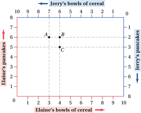
To do this analysis, we use an Edgeworth box. An Edgeworth box utilizes the fact that when there is a fixed total number of goods to be split between two individuals, giving one more unit of a good to one person necessarily means the other person gets one less unit. In our case, for example, if Elaine gets one more bowl of cereal, Jerry must get one less. A point within or on the sides of the Edgeworth box shows the distribution of two goods (like cereal and pancakes) between two people (like Jerry and Elaine).
Figure 15.5 illustrates how the Edgeworth box works in our example. The horizontal sides of the box measure 10 bowls of cereal; the vertical sides measure 8 pancakes. The lower-
592
The upper-
To get accustomed to working with the Edgeworth box, let’s do some quick examples. Consider an initial allocation at point A in Figure 15.5. At point A, Elaine has 3 bowls of cereal and 6 pancakes, and Jerry has the rest of the goods, 7 bowls of cereal and 2 pancakes. If we change the allocation by giving Elaine another bowl of cereal and taking one from Jerry, we are at point B; Elaine has 4 bowls of cereal and 6 pancakes and Jerry has 6 bowls of cereal and 2 pancakes. If we change the allocation from point B by taking away a pancake from Elaine and giving it to Jerry, we move to point C (Elaine has 4 bowls of cereal and 5 pancakes and Jerry has 6 bowls of cereal and 3 pancakes). Any change in the allocation that moves one of the consumers in a certain direction will move the other consumer by the same amount but in the opposite direction. As a result, the Edgeworth box allows us to see simultaneously the effects of changes in goods allocations on both consumers. Think of it as almost a game board where each person’s side is the opposite of the other.
Gains from Trade in the Edgeworth Box
To analyze whether allocations are efficient, we need to know consumers’ preferences. In Chapter 4, we learned that indifference curves show consumers’ preferences. To see the gains from trade, we add Elaine’s and Jerry’s indifference curves to the Edgeworth box (Figure 15.6).
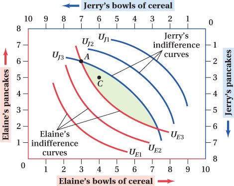
Elaine’s preferences for bowls of cereal and pancakes are represented by indifference curves UE1, UE2, UE3, and so on. Each shows combinations of cereal and pancakes that make Elaine equally well off. Indifference curves farther away from Elaine’s origin depict more of each good, and so represent higher utility levels. Jerry’s preferences are represented by indifference curves UJ1, UJ2, UJ3, and so on. Jerry’s indifference curves may look odd, but when you remember that Jerry’s origin is in the upper right corner, then they look like all other indifference curves: bowed toward the origin. Indifference curves farther away from Jerry’s origin show higher utility levels.
593
Now that we’ve laid out Jerry and Elaine’s preferences, how can we use them to determine what an efficient allocation of the two goods would be? We start at an arbitrary allocation, point A, and ask if we can reshuffle who gets what and make both Elaine and Jerry better off by doing so. (Remember the definition of Pareto efficiency: There is no possible way to reallocate who gets what without making at least one individual worse off than before.) At allocation A, such a reshuffling is possible. Let’s see why.
Elaine and Jerry each have indifference curves that pass through point A, UE3 and UJ3. We know from our analysis in Chapter 4 that any allocation giving Elaine quantities of cereal and pancakes that are above and to the right of UE3 will give her a higher utility than at point A. Similarly, any allocation that raises Jerry’s utility will be below and to the left of UJ3. Knowing this, we can figure out the allocations that make both Elaine and Jerry better off, or at least make one of them better off without making the other worse off. These are the allocations in the shaded area in Figure 15.6. Any distribution of goods in this area must be on indifference curves (not drawn to keep the graph uncluttered) that correspond to higher utility levels for both Elaine and Jerry. Any change that moves the allocation of goods from A to somewhere in the shaded area makes both Elaine and Jerry better off. For example, if we gave one of Jerry’s bowls of cereal to Elaine and one of Elaine’s pancakes to Jerry, we’d be at point C inside the shaded area, and Jerry and Elaine would both have higher utility levels than at the initial allocation (point A).
Remember that a Pareto-
If the existence of a shaded area like that in Figure 15.6 means an allocation isn’t Pareto-
Although C gives both Jerry and Elaine higher utility levels than A, there are still mutually beneficial trades that can be made. These can be seen in Figure 15.7. For example, indifference curves UE4 and UJ4 are Elaine and Jerry’s indifference curves that pass through C. The area that UE4 and UJ4 enclose are cereal and pancake allocations that would make both Elaine and Jerry better off than they are with allocation C. Therefore, allocation C can’t be Pareto-
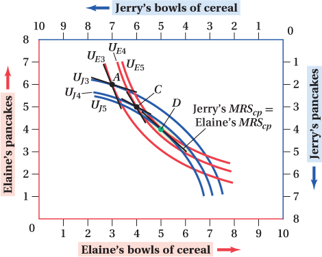
To find a Pareto-
594
We’ve shown that exchange efficiency is achieved when two consumers’ indifference curves are tangent. Only at such a tangency are there no mutually beneficial gains from trade. This tangency condition offers an interpretation for what must be true for exchange efficiency to hold. Recall from Chapter 4 that the slope of an indifference curve at any point reflects the marginal rate of substitution (MRS) between goods at that point. That means at a common tangency like point D, the slopes of both Jerry and Elaine’s indifference curves are the same. (Remember, the slope of a curve at a particular point equals the slope of a line tangent to the curve at that point.) Thus, at point D, Jerry and Elaine have the same MRS between cereal and pancakes. At any point that isn’t a Pareto-
To understand why the MRSs need to be equal, think for a moment about what it would mean if they weren’t. One consumer would have a higher marginal utility from consuming one of the goods than the other consumer would. For the other good, the order of the two consumers’ marginal utilities would be switched. When marginal utilities for the same good are unequal across consumers, each could give a unit of her low-
In allocation A in Figure 15.7, Elaine would be willing to trade 3 pancakes for 1 bowl of cereal. That is, her MRScp (marginal rate of substitution of cereal for pancakes) and the absolute value of the slope of her indifference curve is 3. Jerry would trade 3 bowls of cereal for 1 pancake, or equivalently, one-
595
Prices and the Allocation of Goods Up to this point, we’ve talked about the allocation of goods as if magical economists shuffle goods among consumers. In reality, consumers choose how much of each good to consume given the prices they face. In Chapter 4, we learned that a utility-
In Elaine and Jerry’s case, then, we know that they will both consume amounts where 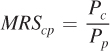 . We also just saw that Elaine and Jerry’s MRScp will be equal in a Pareto-
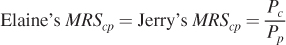
In other words, an efficient market will result in the goods’ price ratio equaling consumers’ marginal rates of substitution for those goods.
If an initial allocation is not efficient, consumers will be willing to sell their allocated goods that (for them) have marginal utilities below the market price. They could then use the proceeds to buy high-
consumption contract curve
Curve that shows all possible Pareto-
The Consumption Contract Curve The key condition of exchange efficiency that consumers’ marginal rates of substitution are equal—
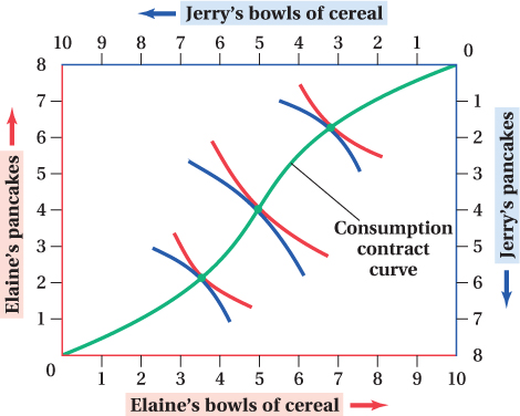
Looking at the contract curve emphasizes the distinction between efficiency and equity that we mentioned earlier. While all allocations along the contract curve are efficient, they have very different implications for Jerry and Elaine’s respective utility levels. Some—
596
figure it out 15.3
For interactive, step-
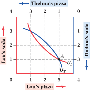
Consider the Edgeworth box above (Figure A), which depicts the amount of soda and pizza available to two consumers, Thelma and Lou.
Suppose that Thelma and Lou are initially at point A. How much soda does each have? How many slices of pizza?
Suppose that Thelma and Lou’s child Ted takes 2 slices of pizza from Lou and gives them to Thelma, then takes 2 sodas from Thelma and gives them to Lou. Find and plot the new allocation in the Edgeworth box. Label the allocation with a large “B.” Does such a reallocation represent a Pareto improvement? Explain your answer.
Suppose that Ted had reallocated 1 slice of pizza and 1 soda instead of 2 of each. Would such a reallocation represent a Pareto improvement? Explain your answer, using indifference curves to illustrate it.
Solution:
At point A, Thelma has 3 sodas and Lou has 1 soda. Thelma has 1 slice of pizza, while Lou has 3 slices of pizza.
If Ted takes 2 slices of pizza from Lou and gives them to Thelma, Lou will end up with 1 slice, while Thelma will have 3. If Ted takes 2 sodas from Thelma and gives them to Lou, Thelma will be left with 1 soda and Lou will have 3 sodas. This allocation can be represented at point B in Figure B. A Pareto improvement occurs when at least one individual is made better off without making anyone worse off. Because point B is on the same indifference curves as point A, neither Thelma nor Lou is better off. Therefore, this is not a Pareto improvement.
 Figure B
If Ted takes 1 slice of pizza from Lou and gives it to Thelma, both Lou and Thelma will end up with 2 slices each. If Ted also takes 1 soda from Thelma and gives it to Lou, both Thelma and Lou will be left with 2 sodas each. This allocation can be represented by point C in Figure C. A Pareto improvement occurs when at least one person is made better off without harming another person. In this case, point C is on a higher indifference curve for both Thelma and Lou, implying that they are both better off with this new allocation. Therefore, it is a Pareto improvement. Moreover, as drawn below, the allocation at point C is also Pareto-
efficient. 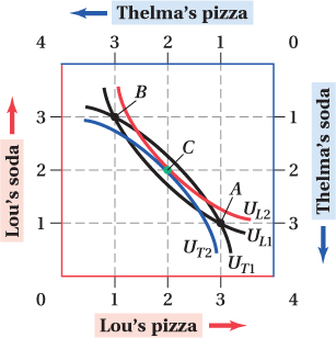 Figure C
597