4.3 The Consumer’s Income and the Budget Constraint
In the preceding sections, we analyzed how a consumer’s preferences can be described by a utility function, why indifference curves are a convenient way to think about utility, and how the slope of the indifference curve—
128
We start looking at the interactions of utility, income, and prices by making some assumptions. To keep things simple, we continue to focus on a model with only two goods.
Each good has a fixed price, and any consumer can buy as much of a good as she wants at that price if she has the income to pay for it. We can make this assumption because each consumer is only a small part of the market for a good, so her consumption decision will not affect the equilibrium market price.
The consumer has fixed income available to spend.
For now, the consumer cannot borrow or save. Without borrowing, she can’t spend more than her income in any given period. With no saving, it means that unspent money is lost forever, so it’s use it or lose it.
budget constraint
A curve that describes the entire set of consumption bundles a consumer can purchase when spending all income.
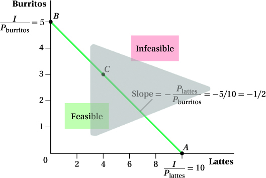
To incorporate prices and the consumer’s income into our model of consumer behavior, we use a budget constraint. This constraint describes the entire set of consumption bundles that a consumer can purchase by spending all of her money. For instance, let’s go back to the example of Sarah and her burritos and lattes. Suppose Sarah has an income of $50 to spend on burritos (which cost $10 each) and lattes ($5 each). Figure 4.14 shows the budget constraint corresponding to this example. The number of lattes is on the horizontal axis; the number of burritos is on the vertical axis. If Sarah spends her whole income on lattes, then she can consume 10 lattes (10 lattes at $5 each is $50) and no burritos. This combination is point A in the figure. If instead Sarah spends all her money on burritos, she can buy 5 burritos and no lattes, a combination shown at point B. Sarah can purchase any combination of burritos and lattes that lies on the straight line connecting these two points. For example, she could buy 3 burritos and 4 lattes. This is point C.
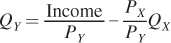
The mathematical formula for a budget constraint is
Income = PXQX + PYQY
129
where PX and PY are the prices for 1 unit of goods X and Y (lattes and burritos in our example) and QX and QY are the quantities of the two goods. The equation simply says that the total expenditure on the two goods (the per-
feasible bundle
A bundle that the consumer has the ability to purchase; lies on or below the consumer’s budget constraint.
infeasible bundle
A bundle that the consumer cannot afford to purchase; lies to the right and above a consumer’s budget constraint.
Any combination of goods on or below the budget constraint (i.e., any point between the origin on the graph and the budget constraint, including those on the constraint itself) is feasible, meaning that the consumer can afford to buy the bundle with her income. Any points above or to the right of the budget line are infeasible. These bundles are beyond the consumer’s reach even if she spends her entire income. Figure 4.14 shows the feasible and infeasible bundles for the budget constraint 50 = 5Qlattes + 10Qburritos.
The budget constraint in Figure 4.14 is straight, not curved, because we assumed Sarah can buy as much as she wants of a good at a set price per unit. Whether buying the first latte or the tenth, we assume the price is the same. As we see later, if the goods’ prices change with the number of units purchased, the budget line will change shape depending on the amount of the goods purchased. That’s an unusual case, though.
The Slope of the Budget Constraint
The relative prices of the two goods determine the slope of the budget constraint. Because the consumer spends all her money when she is on the budget constraint line, if she wants to buy more of one good and stay within her budget, she has to buy less of the other. Relative prices pin down the rate at which purchases of the two goods can be traded off. If she wants to buy 1 more burrito (a cost of $10), for example, she’ll have to buy 2 fewer lattes at $5.
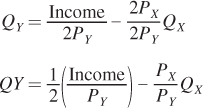
We can see the equivalence between relative prices and the slope of the budget constraint by rearranging the budget constraint:
Income = PXQX + PYQY
PYQY = Income – PXQX
The equation shows if QX—the quantity purchased of good X—increases by 1 unit, the quantity of good Y, or QY, that can be bought falls by PX/PY. This ratio of the price of good X relative to the price of good Y is the negative of the slope of the budget constraint. It makes sense that this price ratio determines the slope of the constraint. If good X is expensive relative to good Y (i.e., PX/PY is large), then buying additional units of X will mean you must give up a lot of Y and the budget constraint line will be steep. If good X is relatively inexpensive, you don’t have to give up a lot of Y to buy more X, and the constraint line will be flat.
We can use the equation for the budget constraint (Income = PXQX + PYQY) to find its slope and intercepts. Using the budget constraint (50 = 5Qlattes + 10Qburritos) shown in Figure 4.14, we get
50 = 5QX + 10QY
10QY = 50 – 5QX
Dividing each side by 10—
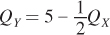
As we noted earlier, if Sarah spends all of her income on lattes, she will buy 10 lattes (the x-intercept), while she can purchase 5 burritos (the y-intercept) using all of her income. These relative prices and intercepts are shown in Figure 4.14.
130
As will become clear when we combine indifference curves and budget constraints in the next section, the slope of the budget constraint plays an incredibly important role in determining which consumption bundles maximize consumers’ utility levels.
Factors That Affect the Budget Constraint’s Position
Because relative prices determine the slope of the budget constraint, changes in relative prices will change its slope. Figure 4.15a demonstrates what happens to our example budget constraint if the price of lattes doubles to $10. The budget constraint rotates clockwise around the vertical axis. Because PX doubles, PX/PY doubles, and the budget constraint becomes twice as steep. If Sarah spends all her money on lattes, then the doubling of the price of lattes means she can buy only half as many lattes with the same income (the 5 lattes shown at A′, rather than 10 lattes as before). If, on the other hand, she spends all her money on burritos (point B), then the change in the price of a latte doesn’t affect the bundle she can consume. That’s because the price of burritos is still the same ($10). Notice that after the price increase, the set of feasible consumption bundles is smaller: There are now fewer combinations of goods that Sarah can afford with her income.
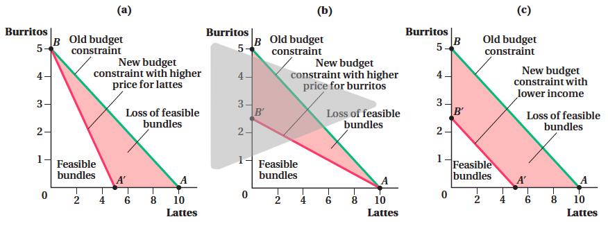
(b) When the price of burritos increases, the vertical intercept (I/Pburritos) falls, the slope (–Plattes/Pburritos) gets flatter, the budget constraint rotates toward the origin, and again, Sarah has a smaller choice set. The higher price for burritos means that she can buy fewer burritos or, for a given purchase of burritos, she has less money available to buy lattes.
(c) When Sarah’s income is reduced, both the horizontal and vertical intercepts fall and the budget constraint shifts in. The horizontal intercept is lower because income I falls; thus, (I/Plattes) falls. The same holds for the vertical axis. Because the movement along both axes is caused by the change in income (the reduction in I is the same along both axes), the new budget constraint is parallel to the initial budget constraint. Given a reduction in income, Sarah’s choice set is reduced.
If, instead, the price of a burritos doubles to $20, but lattes remain at their original $5 price (as in Figure 4.15b), the budget constraint’s movement is reversed: It rotates counterclockwise around the horizontal axis, becoming half as steep. If Sarah wanted to buy only lattes, this wouldn’t affect the number of lattes she could buy. If she wants only burritos, now she can obtain only half as many (if you could buy a half a burrito; we’ll assume you can for now), at bundle B′. Notice that this price increase also shrinks the feasible set of bundles just as the lattes’ price increase did. Always remember that when the price rises, the budget constraint rotates toward the origin. When the price falls, it rotates away from the origin.
131
Now suppose prices are stable but Sarah’s income falls by half (to $25). With only half the income, Sarah can buy only half as many lattes and burritos as she could before. If she spends everything on lattes, she can now buy only 5. If she buys only burritos, she can afford 2.5. But because relative prices haven’t changed, the tradeoffs between the goods haven’t changed. To buy 1 more burrito, Sarah still has to give up 2 lattes. Thus, the slope of the budget constraint remains the same. This new budget constraint is shown in Figure 4.15c.
Note that had both prices doubled while income stayed the same, the budget constraint would be identical to the new one shown in Figure 4.15c. We can see this more clearly if we plug in 2PX and 2PY for the prices in the slope-
In both the figure and the equation, this type of change in prices decreases the purchasing power of the consumer’s income, shifting the budget constraint inward. The same set of consumption bundles is feasible in either case. If Sarah’s income had increased rather than decreased as in our example (or the prices of both goods had fallen in the same proportion), the budget constraint would have shifted out rather than in. Its slope would remain the same, though, because the relative prices of burritos and lattes would not have changed.
We’ve now considered what happens to the budget constraint in two situations: when income changes while prices stay constant and when prices change, holding income constant. If prices and income both go up proportionally (e.g., all prices double and income doubles), then the budget constraint doesn’t change at all. You have double the money but everything costs twice as much, so you can only afford the same bundles you could before. You can see this mathematically in the equation for the budget constraint above: If you multiply all prices and income by any positive number (call it k), all the ks will cancel out, leaving you with the original equation.
figure it out 4.3
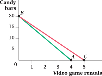
Braden has $20 per week that he can spend on video game rentals (R), priced at $5 per game, and candy bars (C), priced at $1 each.
Write an equation for Braden’s budget constraint and draw it on a graph that has video game rentals on the horizontal axis. Be sure to show both intercepts and the slope of the budget constraint.
Assuming he spends the entire $20, how many candy bars does Braden purchase if he chooses to rent 3 video games?
Suppose that the price of a video game rental falls from $5 to $4. Draw Braden’s new budget line (indicating intercepts and the slope).
Solution:
The budget constraint represents the feasible combinations of video game rentals (R) and candy bars (C) that Braden can purchase given the current prices and his income. The general form of the budget constraint would be Income = PRR + PCC. Substituting in the actual prices and income, we get 20 = 5R + 1C.
To diagram the budget constraint (see the next page), first find the horizontal and vertical intercepts. The horizontal intercept is the point on Braden’s budget constraint where he spends all of his $20 on video game rentals. The x-intercept is at 4 rentals ($20/$5), point A on his budget constraint. The vertical intercept represents the point where Braden has used his entire budget to purchase candy bars. He could purchase 20 candy bars ($20/$1) as shown at point B. Because the prices of candy bars and video game rentals are the same no matter how many Braden buys, the budget constraint is a straight line that connects these two points.
The slope of the budget constraint can be measured by the rise over the run. Therefore, it is equal to
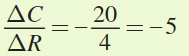 . We can check our work by recalling that the slope of the budget constraint is equal to the negative of the ratio of the two prices or
 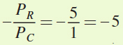 . Remember that the slope of the budget constraint shows the rate at which Braden is able to exchange candy bars for video game rentals.
If Braden currently purchases 3 video game rentals, that means he spends $15 (= $5 × 3) on them. This leaves $5 (= $20 – $15) for purchasing candy bars. At a price of $1 each, Braden purchases 5 candy bars.
When the price of a video game rental falls to $4, the vertical intercept is unaffected. If Braden chooses to spend his $20 on candy bars, at a price of $1, he can still afford to buy 20 of them. Thus, point B will also be on his new budget constraint. However, the horizontal intercept increases from 4 to 5. At a price of $4 per rental, Braden can now afford 5 rentals if he chooses to allocate his entire budget to rentals (point C). His new budget constraint joins points B and C.
The slope of the budget constraint is
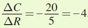 . Note that this equals the inverse price ratio of the two goods
 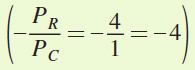 .
.
132
Nonstandard Budget Constraints
In all the examples so far, the budget constraint has been a straight line. There are some cases in which the budget constraint would be kinked instead.
Quantity Discounts Suppose Alex spends his $100 income on pizzas and phone calls. A pizza costs $10; if he spends everything on pizzas, he can buy 10. If the price of phone minutes is constant at 10 cents per minute, he can buy as many as 1,000 minutes of phone time. Figure 4.16 portrays this example graphically. The budget constraint in the case where minutes are priced at a constant 10 cents is given by the solid section of the line running from zero minutes and 10 pizzas up to 1,000 minutes and zero pizzas.
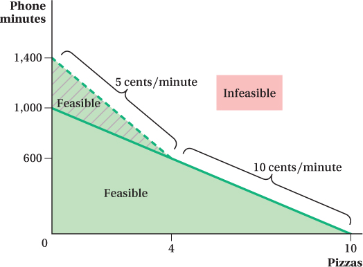
Phone plans often offer quantity discounts on goods such as phone minutes. With a quantity discount, the price the consumer pays per unit of the good depends on the number of units purchased. If Alex’s calling plan charges 10 cents per minute for the first 600 minutes per month and 5 cents per minute after that, his budget constraint will have a kink. In particular, because phone minutes become cheaper above 600 minutes, the actual budget constraint has a kink at 600 minutes and 4 pizzas. Because the price of the good on the y-axis (phone minutes) becomes relatively cheaper, the constraint rotates clockwise at that quantity, becoming steeper. To find where the budget constraint intercepts the vertical axis, we have to figure out how many minutes Alex can buy if he purchases only cell phone time. This total is 1,400 minutes [(600 × $0.10) + (800 × $0.05) = $100]. In Figure 4.16, the resulting budget constraint runs from 10 pizzas and zero minutes to 4 pizzas and 600 minutes (part of the solid line) and then continues up to zero pizzas and 1,400 minutes (the dashed line). It’s clear from the figure that the lower price for phone time above the 600-
133
Quantity Limits Another way a budget constraint can be kinked is if there is a limit on how much of one good can be consumed. When the newest iPhone model comes out, Apple often sets a limit of one per customer. Similarly, during World War II in the United States, certain goods like sugar and butter were rationed. Each family could buy only a limited quantity. And during the oil price spikes of the 1970s, gas stations often limited the amount of gasoline people could buy. These limits have the effect of creating a kinked budget constraint.9
9 Note that limits on how much a consumer can purchase are a lot like the quotas we learned about in Chapter 3, except now they apply to a single consumer, rather than to the market as a whole.
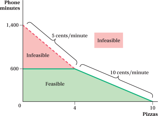
Suppose that the government (or maybe his parents, if he lives at home) dictates that Alex can talk on the phone for no more than 600 minutes per month. In that case, the part of the budget constraint beyond 600 minutes becomes infeasible, and the constraint becomes horizontal at 600 minutes, as shown by the solid line in Figure 4.17. Note that neither Alex’s income nor any prices have changed in this example. He still has enough money to reach any part in the area below the dashed section of the budget constraint that is labeled infeasible. He just isn’t allowed to spend it. Consequently, for the flat part of the budget constraint, he will have unspent money left over. As we see in the next section, you will never actually want to consume a bundle on the flat part of the budget constraint. (You might want to see if you can figure out why yourself, before we tell you the answer.)
134