Cost Minimization Using Calculus
Now that we have verified the usefulness of the Cobb–Douglas function for modeling production, let’s turn to the firm’s cost-minimization problem. Once again, we are faced with a constrained optimization problem: The objective function is the cost of production, and the constraint is the level of output. The firm’s goal is to spend the least amount of money to produce a specific amount of output. This is the producer’s version of the consumer’s expenditure-minimization problem.
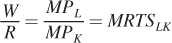
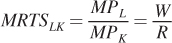
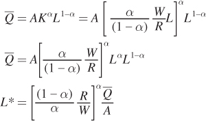
As we saw with the consumer’s problem, there are two approaches to solving the cost-minimization problem. The first is to apply the cost-minimization condition that we derived in the chapter. At the optimum, the marginal rate of technical substitution equals the ratio of the input prices, wages W and capital rental rate R. We just showed that the marginal rate of technical substitution is the ratio of the marginal products, so the cost-minimization condition is
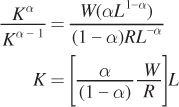
For our Cobb–Douglas production function above, finding the optimum solution is easy using this relationship between the marginal rate of technical substitution and the input prices. We start by solving for K as a function of L using the equation for the marginal rate of technical substitution above:
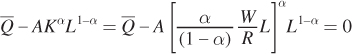
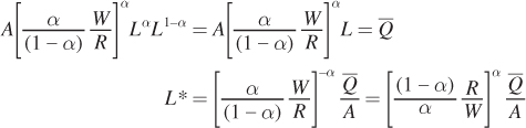
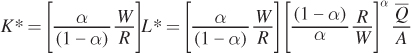
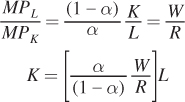
Next, plug K into the production constraint to solve for the optimum quantity of labor L*:
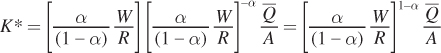
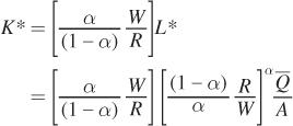
Now solve for K* by plugging L* into the earlier expression for K as a function of L:
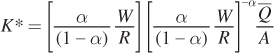
We can simplify this expression by inverting the term in the second set of brackets:
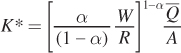
and combining the first and second terms:
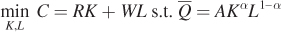
Now let’s use a second approach to solve for the cost-minimizing bundle of capital and labor: the constrained optimization problem. In particular, the firm’s objective, as before, is to minimize costs subject to its production function:
Next, write this constrained optimization problem as a Lagrangian so that we can solve for the first-order conditions:
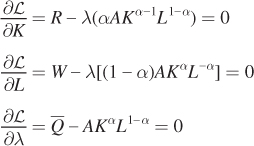
Now take the first-order conditions of the Lagrangian:
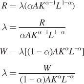
Notice that λ is in both of the first two conditions. Let’s rearrange to solve for λ:
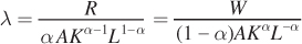
Now set these two expressions for λ equal to one another:
How can we interpret λ in the context of the firm’s cost-minimization problem? In general, the Lagrange multiplier is the value of relaxing the constraint by 1 unit. Here, the constraint is the quantity of output produced; if you increase the given output quantity by 1 unit, the total cost of production at the optimum increases by λ dollars. In other words, λ has a very particular economic interpretation: It is the marginal cost of production, or the extra cost of producing an additional unit of output when the firm is minimizing its costs. We can see that in our λs above: it is the cost of an additional unit of capital (or labor) divided by the additional output produced by that unit. In Chapter 7, we develop other ways to find marginal costs, but it’s good to keep in mind that marginal cost always reflects the firm’s cost-minimizing behavior.
We can get another perspective on cost minimization by inverting the expressions for λ:
This relationship shows us precisely what we know is true at the optimum, that 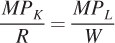 , which we can rearrange to get the cost-minimization condition:
To solve for the optimal bundle of inputs that minimizes cost, we can first solve for K as a function of L:
Plug K as a function of L into the third first-order condition, the constraint:
Now solve for the cost-minimizing quantity of labor, L*:
Substitute L* into our expression for K as a function of L:
To simplify, invert the second term and combine:
So using the Lagrangian, we arrive at the same optimal levels of labor and capital that we found using the cost-minimization condition:
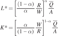
figure it out 6A.1
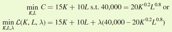
A firm has the production function Q = 20K0.2L0.8, where Q measures output, K represents machine hours, and L measures labor hours. If the rental rate of capital is R = $15, the wage rate is W = $10, and the firm wants to produce 40,000 units of output, what is the cost-minimizing bundle of capital and labor?
We could solve this problem using the cost-minimization condition. But let’s solve it using the Lagrangian, so we can get more familiar with that process. First, we set up the firm’s cost-minimization problem as
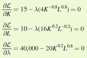
Find the first-order conditions for the Lagrangian:
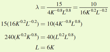
Solve for L as a function of K using the first two conditions:
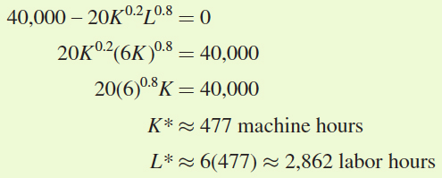
Now plug L into the third first-order condition and solve for the optimal number of labor and machine hours, L* and K*:
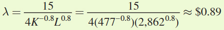
At the optimum, then, the firm will use approximately 477 machine hours and 2,862 labor hours to produce 40,000 units. But once again, the Lagrangian provides us with one additional piece of information: the value of λ, or marginal cost:
Therefore, if the firm wants to produce just one more unit of output—its 40,001st unit of output, to be precise—it would have to spend an additional $0.89.
 units of output is to use
 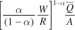 units of capital and
 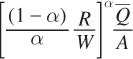 units of labor.