In the long run, firms can change not only their labor inputs but also their capital. This difference gives them two important benefits. First, in the long run, a firm might be able to lessen the sting of diminishing marginal products. As we saw above, when capital is fixed, the diminishing marginal product limits a firm’s ability to produce additional output by using more and more labor. If additional capital can make each unit of labor more productive, then a firm can expand its output more by increasing capital and labor inputs jointly.

Think back to our example of the coffee shop. If the shop adds a second worker per shift when there is only one espresso machine, the firm won’t gain much additional output because of the diminishing marginal product of labor. Hiring still another worker per shift will barely budge output at all. But if the firm bought another machine for each additional worker, output could increase with little drop in productivity. In this way, using more capital and labor at the same time allows the firm to avoid (at least in part) the effects of diminishing marginal products.

The second benefit of being able to adjust capital in the long run is that producers often have some ability to substitute capital for labor or vice versa. Firms can be more flexible in their production methods and in the ways they respond to changes in the relative prices of capital and labor. For example, as airline ticket agents became relatively more expensive and technological progress made automated check-in less so, airlines shifted much of their check-in operations from being labor-intensive (checking in with an agent at the counter) to being capital-intensive (checking in at an automated kiosk or at home online).

In a long-run production function, all inputs can be adjusted. The long-run production is the production function we first introduced in Section 6.2: Q = f(K, L), but rather than having a fixed level of and choosing L (as we did for the short run), now the firm can choose the levels of both inputs.

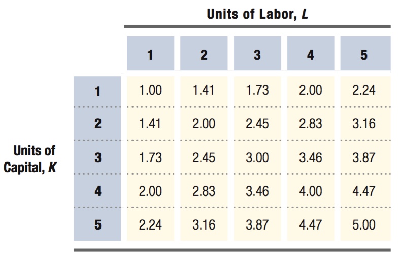
We can also illustrate the long-run production function in a table. Table 6.2 shows the relationship between output and inputs for our example production function Q = K^0.5L^0.5. The columns correspond to different amounts of labor. The rows denote different amounts of capital. The number in each cell is the quantity of output generated by the corresponding combination of inputs.

In the fourth row of the table, where the firm has 4 units of capital, the values exactly match the short-run production function values from Table 6.1. Table 6.1 adds to Table 6.1 other possible output quantities the firm could achieve once it can change its level of capital. One way to think about the long-run production function is as a combination of all the firm’s possible short-run production functions, where each possible short-run function has a different fixed level of capital. Notice that for any given level of capital—that is, for any particular short-run production function—labor has a diminishing marginal product. For example, when capital is fixed at 5 units, the marginal product of labor of the first worker is 2.24, the MP_L of the second worker is 0.92 (= 3.16 – 2.24), the MP_L of the third worker is 0.71 (= 3.87 – 3.16), and so on.

210