6.4 The Firm’s Cost-
cost minimization
A firm’s goal of producing a specific quantity of output at minimum cost.
At the start of the chapter, we made several assumptions about a firm’s production behavior. The third assumption was that the firm’s goal is to minimize the cost of producing whatever quantity it chooses to make. (How a firm determines that quantity is the subject of Chapter 8, Chapter 9, Chapter 10 and Chapter 11.) The challenge of producing a specific amount of a particular good as inexpensively as possible is the firm’s cost-
The firm’s production decision is another constrained optimization problem. Remember from our discussion in Chapter 4 that these types of problems are ones in which an economic actor tries to optimize something while facing a constraint on her choices. Here, the firm’s problem is a constrained minimization problem. The firm wants to minimize the total costs of its production. However, it must hold to a constraint in doing so: It must produce a particular quantity of output. That is, it can’t minimize its costs just by refusing to produce as much as it would like (or refuse to produce anything, for that matter). In this section, we look at how a firm uses two concepts, isoquants (which tell the firm the quantity constraint it faces) and isocost lines (which tell the firm the various costs at which the firm can produce its quantity) to solve its constrained minimization problem.
Isoquants
When learning about the consumer’s utility function in Chapter 4, we looked at three variables: the quantities of the two goods consumed and the consumer’s utility. Each indifference curve showed all the combinations of the two goods consumed that allowed the consumer to achieve a particular utility level.
isoquant
A curve representing all the combinations of inputs that allow a firm to make a particular quantity of output.
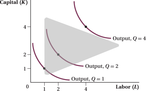
We can do the same thing with the firm’s production function. We can plot as one curve all the possible combinations of capital and labor that can produce a given amount of output. Figure 6.3 does just that for the production function we have been using throughout the chapter; it displays the combinations of inputs that are necessary to produce 1, 2, and 4 units of output. These curves are known as isoquants. (The Greek prefix iso-
211
Just as with indifference curves, isoquants further from the origin correspond to higher output levels (because more capital and labor lead to higher output), isoquants cannot cross (because if they did, the same quantities of inputs would yield two different quantities of output), and isoquants are convex to the origin (because using a mix of inputs generally lets a firm produce a greater quantity than it could by using an extreme amount of one input and a tiny amount of the other).
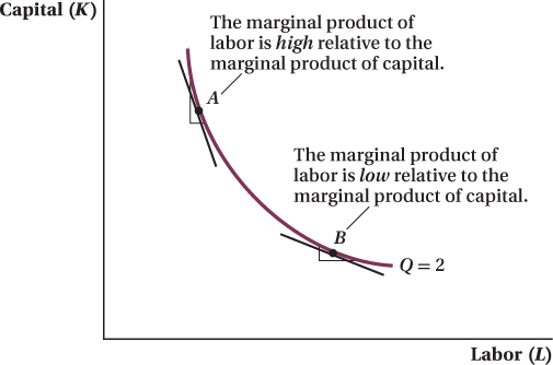
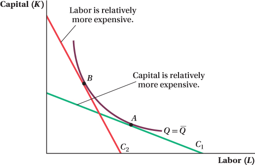
The Marginal Rate of Technical Substitution The slope of the isoquant plays a key role in analyzing production decisions because it captures the tradeoff in the productive abilities of capital and labor. Look at the isoquant in Figure 6.4. At point A, the isoquant is steeply sloped, meaning that the firm can reduce the amount of capital it uses by a lot while increasing labor only a small amount, and still maintain the same level of output. In contrast, at point B, if the firm wants to reduce capital just a bit, it will have to increase labor a lot to keep output at the same level. Isoquants’ curvature and convexity to the origin reflect the fact that the capital–
marginal rate of technical substitution (MRTSXY)
The rate at which the firm can trade input X for input Y, holding output constant.
The negative of the slope of the isoquant is called the marginal rate of technical substitution of one input (on the x-axis) for another (on the y-axis), or MRTSXY. It is the quantity change in input Y necessary to keep output constant if the quantity of input X changes by 1 unit. For the most part in this chapter, we will be interested in the MRTS of labor for capital or MRTSLK, which is the amount of capital needed to hold output constant if the quantity of labor used by the firm changes.
If we imagine moving just a little bit down and to the right along an isoquant, the change in output—
ΔQ = MPL × ΔL + MPK × ΔK = 0
212
∂ The end-of-chapter appendix derives the relationship between the marginal rate of technical substitution and marginal products.
If we rearrange this to find the slope of the isoquant, ΔK/ΔL, we have
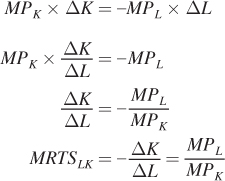
Therefore, the MRTSLK at any point on an isoquant tells you the relative marginal products of capital and labor at that point.
The concepts underlying the marginal rate of technical substitution are the same as those of the marginal rate of substitution (MRS) for consumers, which we learned about in Chapter 4. The two are so closely tied together, in fact, that the names are essentially the same—
The nature of the marginal tradeoffs embodied in the MRS and MRTS implies similar things about the shape of the curves from which they are derived. On the consumer side, indifference curves are convex to the origin because the MRS varies with the amount of each good the consumer is consuming. On the production side, isoquants are convex to the origin because the MRTS varies with the amount of each input the firm uses to produce output. When the firm uses a lot of capital and just a little labor (point A in Figure 6.4), it can replace a lot of capital with a little more labor and still produce the same quantity of output. At this point, labor has a high marginal product relative to capital, and the firm’s isoquant is steep. At point B, the firm uses a lot of labor and only a little capital, so capital has a relatively high marginal product and MRTSLK is small. A smaller MRTSLK means a flatter isoquant at that input mix.
∂ The online appendix explores the relationship between the production function and the shape of isoquants.
Substitutability How curved an isoquant is shows how easily firms can substitute one input for another in production. For isoquants that are almost straight, as in panel a of Figure 6.5, a firm can replace a unit of one input (capital, e.g.) with a particular amount of the second input (labor) without changing its output level, regardless of whether it is already using a lot or a little of capital. Stated in terms of the marginal rate of technical substitution, MRTSLK doesn’t change much as the firm moves along the isoquant. In this case, the two inputs are close substitutes in the firm’s production function, and the relative usefulness of either input for production won’t vary much with how much of each input the firm is using.
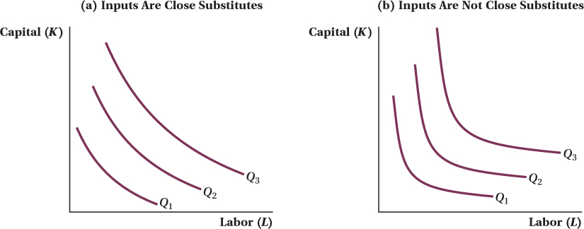
Highly curved isoquants, such as those shown in panel b of Figure 6.5, mean that the MRTSLK changes a lot along the isoquant. In this case, the two inputs are poor substitutes. The relative usefulness of substituting one input for another in production depends a great deal on the amount of the input the firm is already using.
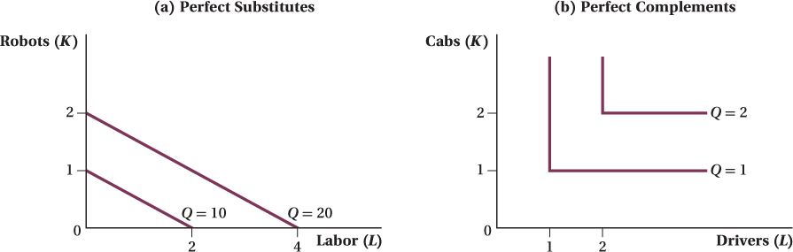
Perfect Substitutes and Perfect Complements in Production In Chapter 4, we discussed the extreme cases of perfect substitutes and perfect complements in consumption. For perfect substitutes, indifference curves are straight lines; for perfect complements, the curves are “L”-shaped right angles. The same holds for inputs: It is possible for them to be perfect substitutes or perfect complements in production. Isoquants for these two cases are shown in Figure 6.6.
213
If inputs are perfect substitutes as in panel a, the MRTS doesn’t change at all with the amounts of the inputs used, and the isoquants are perfectly straight lines. This characteristic means the firm can freely substitute between inputs without suffering diminishing marginal returns. An example of a production function where labor and capital are perfect substitutes is Q = f(K, L) = 10K + 5L; 2 units of labor can always be substituted for 1 unit of capital without changing output, no matter how many units of either input the firm is already using. In this case, imagine that capital took the form of a robot that behaved exactly like a human when doing a task, but did the work twice as quickly as a human. Here, the firm can always substitute one robot for two workers or vice versa, regardless of its current number of robots or workers. This is true because the marginal product of labor is 5 (holding K constant, a 1-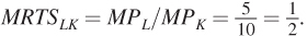
214
If inputs are perfect complements, isoquants have an “L” shape. This implies that using inputs in any ratio outside of a particular fixed proportion—
Isocost Lines
Up to this point in the chapter, we have focused on various aspects of the production function and how quantities of inputs are related to the quantity of output. These aspects play a crucial part in determining a firm’s optimal production behavior, but the production function is only half of the story. As we discussed earlier, the firm’s objective is to minimize its costs of producing a given quantity of output. We’ve said a lot about how the firm’s choices of inputs affect its output but we haven’t talked about the costs of those choices. That’s what we do in this section.
isocost line
A curve that shows all of the input combinations that yield the same cost.
The key concept that brings costs into the firm’s decision is the isocost line. An isocost line connects all the combinations of capital and labor that the firm can purchase for a given total expenditure on inputs. As we saw earlier, iso-
C = RK + WL
where R is the price (the rental rate) per unit of capital, W is the price (the wage) per unit of labor, and K and L are the number of units of capital and labor that the firm hires. It’s best to think of the cost of capital as a rental rate in the same type of units as the wage (e.g., per hour, week, or year). Because capital is used over a long period of time, we can consider R to be not just the purchase price of the equipment but also the economic user cost of capital. The user cost takes into account capital’s purchase price, as well as its rate of depreciation and the opportunity cost of the funds tied up in its purchase (foregone interest).
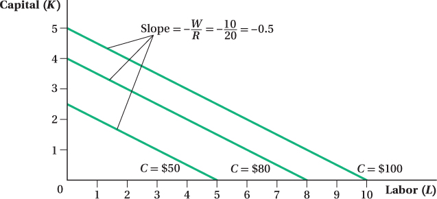
Figure 6.7 shows isocost lines corresponding to total cost levels of $50, $80, and $100, when the price of capital is $20 per unit and labor’s price is $10 per unit. There are a few things to notice about the figure. First, isocost lines for higher total expenditure levels are further from the origin. This reflects the fact that, as a firm uses more inputs, its total expenditure on those inputs increases. Second, the isocost lines are parallel. They all have the same slope, regardless of what total cost level they represent. To see why they all have the same slope, let’s first see what that slope represents.
 . Therefore, for every 1-
215
We can rewrite the equation for the isocost line in slope-
C = RK + WL
RK = C – WL
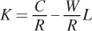
This means that the y-intercept of the isocost line is C/R, while the slope is the (negative of the) inputs’ price ratio, –W/R.
As is so often the case in economics, the slope tells us about tradeoffs at the margin. Here, the slope reflects the cost consequences of trading off or substituting one input for another. It indicates how much more of one input a firm could hire, without increasing overall expenditure on inputs, if it used less of the other input. If the isocost line’s slope is steep, labor is relatively expensive compared to capital. If the firm wants to hire more labor without increasing its overall expenditure on inputs, it is going to have to use a lot less capital. (Or if you’d rather, if it chose to use less labor, it could hire a lot more capital without spending more on inputs overall.) If the price of labor is relatively cheap compared to capital, the isocost line will be relatively flat. The firm could hire a lot more labor and not have to give up much capital to do so without changing expenditures.
Because of our assumption (Assumption 8) that the firm can buy as much capital or labor as it wants at a fixed price per unit, the slopes of isocost lines are constant. That’s why they are straight, parallel lines: Regardless of the overall cost level or the amount of each input the firm chooses, the relative tradeoff between the inputs in terms of total costs is always the same.
If these ideas seem familiar to you, it’s because the isocost line is analogous to the consumer’s budget line we saw in Chapter 4. The consumer’s budget line expressed the relationship between the quantities of each good consumed and the consumer’s total expenditure on those goods. Isocost lines capture the same idea, except with regard to firms and their input purchases. We saw that the negative of the slope of the consumer’s budget constraint was equal to the price ratio of the two goods, just as the negative of the slope of the isocost line equals the price ratio of the firm’s two inputs.
216
Isocost Lines and Input Price Changes Just like budget lines for consumers, when relative prices change, the isocost line rotates. In our example, say labor’s price (W) rose from $10 to $20. Now if the firm only hired labor, it would only be able to hire half as much. The line becomes steeper as in Figure 6.8. The isocost line rotates because its slope is –W/R. When W increases from $10 to $20, the slope changes from
to –1, and the isocost line rotates clockwise and becomes steeper.
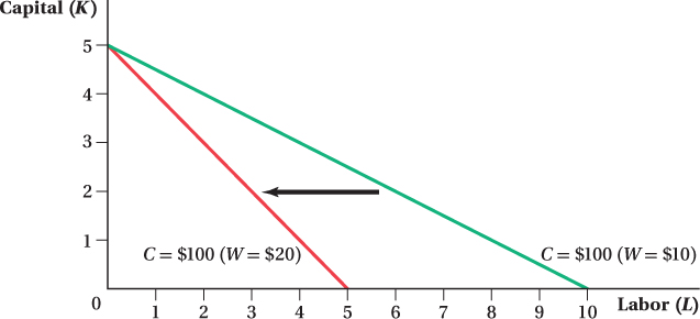
 , or –1. The isocost line, therefore, becomes steeper, and the quantity of inputs the firm can buy for $100 decreases.
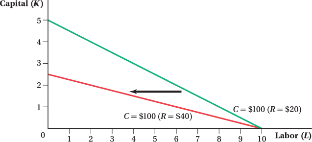
Changes in the price of capital also rotate the isocost line. Figure 6.9 shows what happens to the $100 isocost line when the price of capital increases from $20 to $40 per unit, and the wage stays at $10 per unit of labor. If the firm hired only capital, it could afford half as much, so the slope flattens. A drop in the capital price would rotate the isocosts the other way.
 to
to  . The quantity of inputs the firm can buy for $100 decreases and the isocost line becomes flatter.
217
figure it out 6.2
Suppose that the wage rate is $10 per hour and the rental rate of capital is $25 per hour.
Write an equation for the isocost line for a firm.
Draw a graph (with labor on the horizontal axis and capital on the vertical axis) showing the isocost line for C = $800. Indicate the horizontal and vertical intercepts along with the slope.
Suppose the price of capital falls to $20 per hour. Show what happens to the C = $800 isocost line including any changes in intercepts and the slope.
Solution:
An isocost line always shows the total costs for the firm’s two inputs in the form of C = RK + WL. Here, the wage rate (W) is $10 and the rental rate of capital (R) is $25, so the isocost line is C = 10L + 25K.
We can plot the isocost line for C = $800 = 10L + 25K. One easy way to do this is to compute the horizontal and vertical intercepts. The horizontal intercept tells us the amount of labor the firm could hire for $800 if it only hired labor. Therefore, the horizontal intercept is $800/W = $800/$10 = 80. The vertical intercept tells us how much capital the firm could hire for $800 if it were to use only capital. Thus, it is $800/R = $800/$25 = 32. We can plot these points on the following graph and then draw a line connecting them. This is the C = $800 isocost line labeled C1.
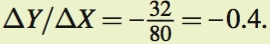
We can calculate slope in several different ways. First, we can simply calculate the slope of the isocost line as drawn. Remember that the slope of a line is ΔY/ΔX (i.e., rise over run). Therefore, the slope is
 We can also rearrange our isocost line into slope-
intercept form by isolating K: 800 = 10L + 25K
25K = 800 – 10L
K = (800/25) – (10/25)L = 32 – 0.4L
This equation tells us that the vertical intercept is 32 (which we calculated earlier) and –0.4 is the slope.
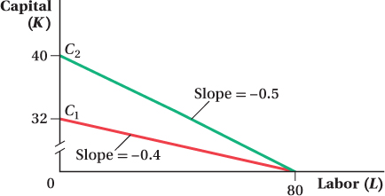
If R falls to $20, the horizontal intercept is unaffected. If the firm is only using labor, a change in the price of capital will have no impact. However, the vertical intercept rises to $800/R = $800/$20 = 40 and the isocost line becomes steeper (C2). The new slope is –W/R = –$10/$20 = –0.5.
Identifying Minimum Cost: Combining Isoquants and Isocost Lines
As we have discussed, a firm’s goal is to produce its desired quantity of output at the minimum possible cost. In deciding how to achieve this goal, a firm must solve a cost-
218
Cost Minimization—
We can combine information about the firm’s costs and the firm’s production function on the same graph to analyze its decision. The isocost lines show the firm’s costs. Then to represent the firm’s production function, we plot the isoquants. These tell us, for a given production function, how much capital and labor it takes to produce a fixed amount of output.
Before we work through a specific example, think about the logic of the firm’s cost- . The cost-
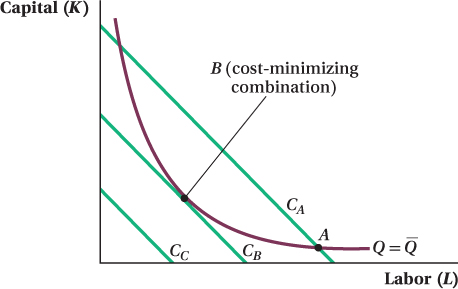
 . Figure 6.10 shows the isoquant for the firm’s desired output quantity
. The firm wants to produce this quantity at minimum cost. How much capital and labor should it hire to do so? Suppose the firm is considering the level inputs shown at point A, which is on isocost line CA. That point is on the
. Figure 6.10 shows the isoquant for the firm’s desired output quantity
. The firm wants to produce this quantity at minimum cost. How much capital and labor should it hire to do so? Suppose the firm is considering the level inputs shown at point A, which is on isocost line CA. That point is on the  isoquant, so the firm will produce the desired level of output. However, there are many other input combinations on the
isoquant that are below and to the left of CA. These all would allow the firm to produce
but at lower cost than input mix A. Only one input combination exists that is on the
isoquant but for which there are no other input combinations that would allow the firm to produce the same quantity at lower cost. That combination is at point B, on isocost CB. There are input combinations that involve lower costs than B—for example, any combination on isocost line CC—but these input levels are all too small to allow the firm to produce
.
isoquant, so the firm will produce the desired level of output. However, there are many other input combinations on the
isoquant that are below and to the left of CA. These all would allow the firm to produce
but at lower cost than input mix A. Only one input combination exists that is on the
isoquant but for which there are no other input combinations that would allow the firm to produce the same quantity at lower cost. That combination is at point B, on isocost CB. There are input combinations that involve lower costs than B—for example, any combination on isocost line CC—but these input levels are all too small to allow the firm to produce
.
 . Because A is on the isoquant, the firm can choose to use input combination A to produce
. However, A is not cost-
at a lower cost at any point below and to the left of the isocost CA. Point B, located at the tangency between isocost CB and the isoquant, is the firm’s cost-
.
. Because A is on the isoquant, the firm can choose to use input combination A to produce
. However, A is not cost-
at a lower cost at any point below and to the left of the isocost CA. Point B, located at the tangency between isocost CB and the isoquant, is the firm’s cost-
.
The total costs of producing a given quantity are minimized where the isocost line is tangent to the isoquant. Point B is the point of tangency of the isocost line CB to the
isoquant.
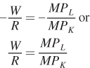
With this tangency property, we once more see a similarity to optimal consumer behavior, which was also identified by a point of tangency. Another important feature of the tangency result is that the isocost line and isoquant have the same slope at a tangency point (that’s the definition of a tangency point). We know what these slopes are from our earlier discussion. The slope of the isocost line is the negative of the relative price of the inputs, –W/R. For the isoquant, the slope is the negative of the marginal rate of technical substitution (MRTSLK), which is equal to the ratio of MPL to MPK. The tangency therefore implies that at the combination of inputs that minimizes the cost of producing a given quantity of output (like point B), the ratio of input prices equals the MRTS:
219
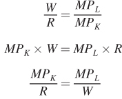
This condition has an important economic interpretation that might be easier to see if we rearrange the condition as follows:
∂ The end-of-chapter appendix uses calculus to solve the firm’s cost-minimization problem.
The way we’ve written it, each side of this equation is the ratio of an input’s marginal product to its price (capital on the left, labor on the right). One way to interpret these ratios is that they measure the marginal product per dollar spent on each input, or the input’s “bang for the buck.” Alternatively, we can think of each of these ratios as the firm’s marginal benefit-
Why does cost minimization imply that each input’s benefit-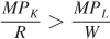 , then the firm’s benefit-
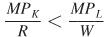 , the firm could reduce the costs of producing its current quantity (or raise its production without increasing costs) by substituting labor for capital because the marginal product per dollar spent is higher for labor. Only when the benefit-
Again, this logic parallels that from the consumer’s optimal consumption choice in Chapter 4. There, at the optimal point the marginal rate of substitution between goods equals the goods’ price ratio. Here, the analog to the MRS is the MRTS (the former being a ratio of marginal utilities, the latter a ratio of marginal products), and the price ratio is now the input price ratio.
There is one place where the parallel between consumers and firms is not exact. The budget constraint plays a big role in the consumer’s utility-
220
Input Price Changes
We’ve established that the cost-
figure it out 6.3
For interactive, step-
A firm is employing 100 workers (W = $15/hour) and 50 units of capital (R = $30/hour). At the firm’s current input use, the marginal product of labor is 45 and the marginal product of capital is 60. Is the firm producing its current level of output at the minimum cost or is there a way for the firm to do better? Explain.
Solution:
The cost-
MPL = 45 and W = 15, so MPL/W = 45/15 = 3
MPK = 60 and R = 30, so MPK/R = 60/30 = 2
Therefore, MPL/W > MPK/R. The firm is not currently minimizing its cost.
Because MPL/W > MPK/R, $1 spent on labor yields a greater marginal product (i.e., more output) than $1 spent on capital. The firm would do better by reducing its use of capital and increasing its use of labor. Note that as the firm reduces capital, the marginal product of capital will rise. Likewise, as the firm hires additional labor, the marginal product of labor will fall. Ultimately, the firm will reach its cost-
A Graphical Representation of the Effects of an Input Price Change We saw that differences in input costs show up as differences in the slopes of the isocost lines. A higher relative cost of labor (from an increase in W, decrease in R, or both) makes isocost lines steeper. Decreases in labor’s relative cost flatten them. A cost-
Figure 6.11 shows an example of this. The initial input price ratio gives the slope of isocost line C1. The firm wants to produce the quantity
, so initially the cost-
221
The implication of this outcome makes sense: If a firm wants to minimize its production costs and a particular input becomes relatively more expensive, the firm will substitute away from the now more expensive input toward the relatively less expensive one.
∂ The online appendix derives the firm’s demands for capital and labor.
This is why we sometimes observe different production methods used to make the same products. For example, if you spend a growing season observing a typical rice-
Application: Hospitals’ Input Choices and Medicare Reimbursement Rules
Medicare is the government-
222
5Daron Acemoglu and Amy Finkelstein, “Input and Technology Choices in Regulated Industries: Evidence from the Health Care Sector,” Journal of Political Economy 116, no. 5 (2008): 837 – 880.
In a study, economists Daron Acemoglu and Amy Finkelstein looked at how changes in Medicare payment structures affect health-
The shift to PPS changed this reimbursement approach. Capital expenses—
Our cost-
When Acemoglu and Finkelstein looked at the capital-
Acemoglu and Finkelstein even identified the types of capital that the hospitals bought: Hospitals with a large fraction of Medicare patients purchased more advanced medical technologies like CT scanners, cardiac-
The production model of this chapter, despite its simplifications, can therefore function as a good predictor of actual firms’ choices in the real world. 
223