Cost Differences and Economic Rent in Perfect Competition
Returns to specialized inputs above what firms paid for them.
In looking at long-run outcomes in perfectly competitive markets, however, we’ve assumed that all firms in an industry had the same cost curves. That’s not very realistic. Firms differ in their production costs for many reasons: They might face different prices for their inputs; they might have various degrees of special know-how that makes them more efficient; or they might have a superior location or access to superior resources. When there are cost differences between firms in a perfectly competitive industry, the more efficient producers earn a special type of return called economic rent.
We saw in Section 8.3 that cost differences among firms is one of the reasons why industry marginal cost curves (and therefore their short-run supply curves) slope up. Higher-cost firms produce only when the market price is high.
To see what happens in the long run when firms have different cost curves, let’s first think about how output quantities vary when firms’ costs do. If all firms have the same cost, their marginal cost curves are the same. Therefore, their profit-maximizing outputs are the same, too: the quantity at which the market price equals (their common) marginal cost. But if firms have different marginal cost curves, their profit-maximizing outputs will differ as well.
Consider an example in which the factors that cause these firms’ costs to differ are specific fixtures of the firm; that is, these costs can’t be influenced by the firm’s actions or sold to other firms. For instance, the factors might involve access to special technologies no one else has or could use if they were sold. In any case, these factors affect only the cost structure of that particular firm. Figure 8.19 shows the long-run marginal cost curves for three firms. Firm 1 has a high marginal cost shown by curve LMC1, Firm 2 has a moderate marginal cost LMC2, and Firm 3 has a low marginal cost LMC3. Each firm’s marginal cost curve intersects the market price at a different quantity of output. Firm 1’s profit-maximizing output is the smallest, Q*1. The next largest is Firm 2, which produces Q*2. Finally, Firm 3 produces the highest output Q*3. Therefore, higher-cost firms produce less, and lower-cost firms produce more, when firms have different costs. This negative relationship between a firm’s size (measured by its output) and its cost has been observed in many industries and countries.
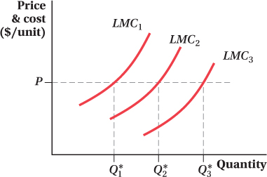
Figure 8.19: Figure 8.19 Firms with Different Long-Run Marginal Costs
Figure 8.19: Firms in the same industry with differing long-run marginal costs will produce different quantities of output at the market price. Because each firm maximizes profit where P = LMC, low-cost producers will produce a greater quantity of output (Q*3) than high-cost producers (Q*1).
Think about the industry’s highest-cost firm, Firm 1. Assume that the market price exceeds Firm 1’s minimum average total cost. As we discussed above, if all producers have the same cost curve, a perfectly competitive market in which price is above the minimum average total cost will attract new entrants. These entrants shift the industry supply curve out and reduce the price until it equals the minimum average total cost. That’s exactly what would happen here, too: If the market price is above Firm 1’s minimum average total cost, the price is above all producers’ minimum average total costs. Therefore, new firms will enter the market. If all these firms have lower costs than Firm 1, the industry supply curve will shift out until the price falls to the minimum average total cost of Firm 1.
If, on the other hand, some entrants have costs above Firm 1’s cost, entry will occur until the supply curve shifts out only enough to lower the price to the minimum average total cost of the highest cost entrant.
In either case, the important thing to realize is that in a perfectly competitive market where firms have different costs, the long-run market price equals the minimum average total cost of the highest-cost firm remaining in the industry. That highest-cost firm makes zero profit and zero producer surplus. The other firms have minimum average total costs that are lower than the minimum average total cost of the highest-cost firm, and therefore lower than the market price. They make a positive profit on every sale, and this profit is larger the lower their costs. It’s just like what we saw in the earlier Application on electricity in Texas: the market price was determined by the marginal cost of the marginal producer, and the lower-cost generating plants could make extra producer surplus at that price. You might wonder why more firms with costs less than those of the highest-cost firm in the market don’t enter. Well, they would . . . if they existed. By entering, they could make a positive margin over their average total cost on every sale. Their entry could shift the industry supply curve out and drive down price enough so that the formerly highest-cost firm in the industry would no longer want to operate because the long-run price would be below its minimum average total cost. Entry would occur, in fact, until there are no more firms left to enter that have costs below those of the industry’s highest-cost firm. Note that if an existing low-cost firm can expand capacity at the existing low-cost level, that’s a different form of entry but is entry nonetheless.
The long-run outcome in an industry in which firms have different costs occurs once all entry has stopped. All firms except the one on the margin (the one with the highest cost but still producing) sell their output at a price above their long-run average total costs, so they all earn producer surplus and economic rent. This surplus is tied to their special attributes that allow them to produce at a lower cost. As we said earlier, their lower cost could be the result of access to a special technology, better know-how of some sort or another, a better location, or a number of other possibilities. The greater this cost advantage is, the larger the producer surplus or economic rent.
Economic rents measure returns to specialized inputs above what the firms paid for them. Suppose a firm is a lower-cost firm because it was lucky enough to have hired a manager who is particularly smart at efficiently running it. If the firm only needed to pay this manager the same salary as every other firm was paying its manager (or, at least not so much more as to wipe out the cost advantage of the manager’s ability), and if there is a limited supply of similarly exceptional managers, the manager’s human capital earns economic rent for the firm. If the firm is instead lower-cost because it has a favorable location that makes servicing customers easier, like a gas station right off a busy highway, the location is the source of economic rent to the firm because not all firms can use that same location. What’s important to recognize is that economic rents are determined by cost differences relative to other firms in the industry. That’s because the profit earned by the scarce input depends on how much lower the firm’s costs are than its competitors’ costs. The larger the cost difference, the larger the rent.
Economic Profit ≠ Economic Rent At this point, you might be a little confused: Earlier we said that perfectly competitive markets had zero economic profit in the long run, yet now we’re saying that firms earn economic rents if they have different costs. Does the zero economic profit outcome only occur if all producers’ costs are the same?
Firms in perfectly competitive industries make zero economic profit even if they have different costs. There is a distinction between economic profit and economic rent. Economic profit counts inputs’ opportunity costs, and economic rent is included in the opportunity cost for inputs that earn them. This is because inputs that earn rents would still earn them if they were given to another firm. If we gave another firm the brilliant manager or the better location discussed above, it would lower that firm’s costs. That other firm would therefore be willing to pay more for that rent-earning input. This willingness to pay for the economic rent inherent to the input raises the opportunity cost of the input to the firm that currently owns it—by using the input, they’re giving up the ability to sell it to another firm. Once this opportunity cost is subtracted from the firm’s revenue, its economic profit is no higher than if the input earned no rent at all.
In practice, this is often hugely important. If one firm has lower costs because it has better programmers and engineers than a different firm, the wages paid to the scarce talent may very well end up absorbing the advantage. The rent in such a case goes to the owner of the scarce resource itself (the workers) rather than to the firm.