9.4 How a Firm with Market Power Reacts to Market Changes
We are now aware how profit-
352
Response to a Change in Marginal Cost
Let’s first think about the effect of an increase in marginal cost. In the iPad example, marginal cost was constant at $200 and the inverse demand curve was P = 1,000 – 5Q (where Q is in millions). Suppose there’s a fire in the plant that manufactures the screen on the iPad, raising the marginal cost of screens, and as a result, the marginal cost of the iPad increases from $200 to $250. What will happen in the market for iPads?
To determine the market impact of this increase in marginal cost, we follow the three-
Step 1: Derive the marginal revenue curve. The demand curve hasn’t changed, so this is the same as before: MR = 1,000 – 10Q.
Step 2: Find the quantity at which MR = MC. The MC is now $250, so
1,000 – 10Q = 250
750 = 10Q
Q* = 75
The new profit-
Step 3: Determine the profit-
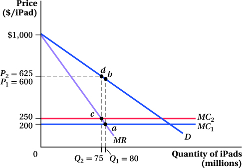
We illustrate the change from the initial equilibrium to the new one in Figure 9.4. The initial quantity of 80 million is set by MR = MC1 ($200) at point a. This quantity corresponds to a price of $600, as indicated at point b. After the fire, the marginal cost curve shifts up to $250 (MC2). Because the fire only affects the supply side of the market, the consumer’s willingness to pay does not change, and the demand and marginal revenue curves do not shift. Now marginal revenue equals marginal cost at point c, at a quantity of 75 million. Following that quantity up to the demand curve (at point d), we can see that the price of an iPad will rise to $625.
353
A firm with market power responds to a cost shock in a way that is similar to a competitive firm’s response. When marginal cost rises, price rises, and output falls. When marginal cost falls, price falls, and output rises.
But in competition, a change in marginal cost is fully reflected in the market price, because P = MC. That doesn’t have to be the case when the seller has market power. In the iPad example, the market price rose only $25 in response to a $50 increase in marginal cost. To maximize its profit, Apple does not want to pass along the full increase in its cost to its customers. The drop in quantity that results from the increase in cost is also smaller than the drop that would occur in a perfectly competitive market. Note, however, that the equilibrium quantity is still higher in a competitive market than one with market power, even after the cost increase. It’s the change in Q that is smaller.6
Response to a Change in Demand
Now suppose that instead of a cost shift, there is a parallel shift in the demand curve. Perhaps a revision of the iPad’s OS doubles battery life, increasing demand and shifting out the demand curve. Specifically, let’s say the new inverse demand curve is P = 1,400 – 5Q. How would the market react to this change?
Again, we follow the three-
MR = 1,400 – 10Q
Setting this equal to the marginal cost (which we’ll assume is back at its original level of $200) implies
1,400 – 10Q = 200
10Q = 1,200
Q* = 120
The quantity produced after the demand shift is now 120 million units, up from 80 million. Finally, we find the new price by plugging this quantity into the inverse demand curve:
P* = 1,400 – 5Q*
= 1,400 – 5(120)
= 800
The new price is $800, up from $600 before the demand shift.
An outward demand shift leads to an increase in both quantity and price in a market where the seller has market power, the same direction as in perfect competition. But again, the size of the changes differs.
354
 See the problem worked out using calculus
figure it out 9.3
For interactive, step-
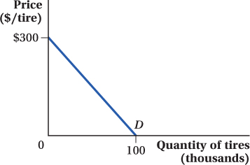
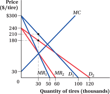
The Power Tires Company has market power and faces the demand curve shown in the figure below. The firm’s marginal cost curve is MC = 30 + 3Q.
What is the firm’s profit-
maximizing output and price? If the firm’s demand changes to P = 240 – 2Q while its marginal cost curve remains the same, what is the firm’s profit-
maximizing level of output and price? How does this compare to your answer for (a)? Draw a diagram showing these two outcomes. Holding marginal cost equal, how does the shape of the demand curve affect the firm’s ability to charge a high price?
Solution:
To solve for the firm’s profit-
maximizing level of output, we need to find the firm’s marginal revenue curve. But, we only have a diagram of the demand curve. So, we will start by solving for the inverse demand function. The inverse demand function will typically have the form P = a – bQ
where a is the vertical intercept and b is the absolute value of the slope
 . We can see from the figure of the demand curve that a = 300. In addition, we can calculate the absolute value of the slope of the demand curve as
 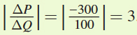 . Therefore, b = 3. This means that the demand for Power Tires is
P = 300 – 3Q
We know that the equation for marginal revenue (when demand is linear) is P = a – 2bQ. Therefore,
MR = 300 – 6Q
Setting marginal revenue equal to marginal cost, we find
MR = MC
300 – 6Q = 30 + 3Q
270 = 9Q
Q* = 30
To find price, we substitute Q = 30 into the firm’s demand equation:
P = 300 – 3Q
= 300 – 3(30) = 210
The firm should produce 30,000 tires and sell them at a price of $210.
If demand changes to P = 240 – 2Q, marginal revenue becomes MR = 240 – 4Q because now a = 240 and b = 2. Setting MR = MC, we find
240 – 4Q = 30 + 3Q
210 = 7Q
Q* = 30
Even with changed demand, the firm should still produce 30 units if it wants to maximize profit. Substituting into the new demand curve, we can see that the price will be
P* = 240 – 2Q*
= 240 – 2(30) = 180
Here, the equilibrium price is lower even though the profit-
maximizing output is the same. The new diagram appears below. Because D2 is flatter than D1, the firm must charge a lower price. Consumers are more responsive to price.
355
The Big Difference: Changing the Price Sensitivity of Customers
One type of market change to which firms with market power react very differently from competitive firms is a change in the price sensitivity of demand—
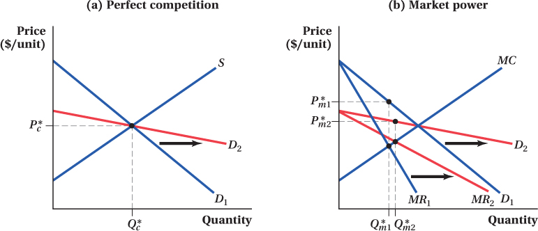
(b) For a firm with market power, a rotation in the demand curve from D1 to D2 rotates the marginal revenue curve from MR1 to MR2. Prior to the rotation, the profit-
Things are different, though, if the same demand curve rotation happens in a market in which there is a seller with market power. That’s because with market power, the rotation in demand also moves the marginal revenue curve as shown in panel b of Figure 9.5. Even though the new demand curve D2 crosses the marginal cost curve at the same quantity as the old demand curve, MR2 intersects the marginal cost curve at a higher quantity than did MR1 ( Q*m2 instead of Q*m1). Therefore, the firm’s output rises as a result of the demand curve rotation and the price falls.
The opposite pattern holds when consumers become less price-
356