A.2 Converting Scores for Purposes of Comparison
Are you taller than you are heavy? That sounds like a silly question, and it is. Height and weight are two entirely different measures, and comparing them is like the proverbial comparison of apples and oranges. But suppose we worded the question this way: Relative to other people of your gender and age group, do you rank higher in height or in weight? Now that is an answerable question. Similarly, consider this question: Are you better at mathematical or at verbal tasks? This, too, is meaningful only if your mathematical and verbal skills are judged relative to those of other people. Compared to other people, do you rank higher in mathematical or in verbal skills? To compare different kinds of scores with each other, we must convert each score into a form that directly expresses its relationship to the whole distribution of scores from which it came.
A6
Percentile Rank
The most straightforward way to see how one person compares to others on a given measure is to determine the person’s percentile rank for that measure. The percentile rank of a given score is simply the percentage of scores that are equal to that score or lower, out of the whole set of scores obtained on a given measure. For example, in the distribution of scores in Table A.1, the score of 37 is at the 25th percentile because 5 of the 20 scores are at 37 or lower ( = ¼ = 25 percent). As another example in the same distribution, the score of 73 is at the 90th percentile because 18 of the 20 scores are lower (
 =
=  = 90 percent). If you had available the heights and weights of a large number of people of your age and gender, you could answer the question about your height compared to your weight by determining your percentile rank on each. If you were at the 39th percentile in height and the 25th percentile in weight, then, relative to others in your group, you would be taller than you were heavy. Similarly, if you were at the 94th percentile on a test of math skills and the 72nd percentile on a test of verbal skills, then, relative to the group who took both tests, your math skills would be better than your verbal skills.
Standardized Scores
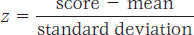
Another way to convert scores for purposes of comparison is to standardize them. A standardized score is one that is expressed in terms of the number of standard deviations that the original score is from the mean of original scores. The simplest form of a standardized score is called a z score. To convert any score to a z score, you first determine its deviation from the mean (subtract the mean from it), and then divide the deviation by the standard deviation of the distribution. Thus,
For example, suppose you wanted to calculate the z score that would correspond to the test score of 54 in the first set of scores in Table A.4. The mean of the distribution is 50, so the deviation is 54 − 50 = +4. The standard deviation is 5.0. Thus, z =  = +0.80. Similarly, the z score for a score of 42 in that distribution would be
  =
=  = −1.60. Remember, the z score is simply the number of standard deviations that the original score is away from the mean. A positive z score indicates that the original score is above the mean, and a negative z score indicates that it is below the mean. A z score of +0.80 is 0.80 standard deviation above the mean, and a z score of −1.60 is 1.60 standard deviations below the mean.
Other forms of standardized scores are based directly on z scores. For example, College Board (SAT) scores were originally (in 1941) determined by calculating each person’s z score, then multiplying the z score by 100 and adding the result to 500. That is,
SAT score = 500 + 100(z)
Thus, a person who was directly at the mean on the test (z = 0) would have an SAT score of 500; a person who was 1 standard deviation above the mean (z = +1) would have an SAT score of 600; a person who was 2 standard deviations above the mean would have 700; and a person who was 3 standard deviations above the mean would have 800. (Very few people would score beyond 3 standard deviations from the mean, so 800 was set as the highest possible score.) Going the other way, a person who was 1 standard deviation below the mean (z = −1) would have an SAT score of 400, and so on. (Today, a much broader range of people take the SAT tests than in 1941, when only a relatively elite group applied to colleges, and the scoring system has not been restandardized to maintain 500 as the average score. The result is that average SAT scores are now considerably less than 500.)
A7
Wechsler IQ scores (discussed in Chapter 10) are also based on z scores. They were standardized—separately for each age group—by calculating each person’s z score on the test, multiplying that by 15, and adding the product to 100. Thus,
IQ = 100 + 15(z)
This process guarantees that a person who scores at the exact mean achieved by people in the standardization group will have an IQ score of 100, that one who scores 1 standard deviation above that mean will have a score of 115, that one who scores 2 standard deviations above that mean will have a score of 130, and so on.
Relationship of Standardized Scores to Percentile Ranks
If a distribution of scores precisely matches a normal distribution, one can determine percentile rank from the standardized score, or vice versa. As you recall, in a normal distribution the highest frequency of scores occurs in intervals close to the mean, and the frequency declines with each successive interval away from the mean in either direction. As illustrated in Figure A.4, a precise relationship exists between any given z score and the percentage of scores that fall between that score and the mean.
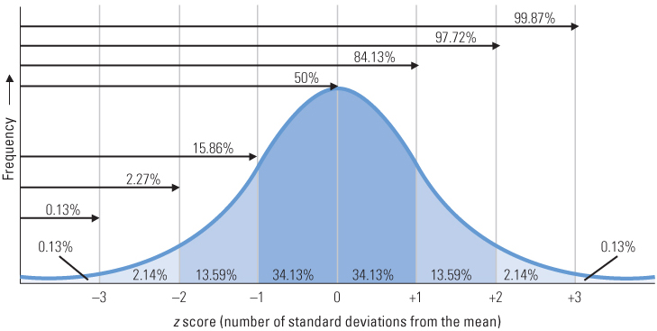
As you can see in the figure, slightly more than 34.1 percent of all scores in a normal distribution will be between a z score of +1 and the mean. Since another 50 percent will fall below the mean, a total of slightly more than 84.1 percent of the scores in a normal distribution will be below a z score of +1. By using similar logic and examining the figure, you should be able to see why z scores of −3, −2, −1, 0, +1, +2, and +3, respectively, correspond to percentile ranks of about 0.1, 2.3, 15.9, 50, 84.1, 97.7, and 99.9, respectively. Detailed tables have been made that permit the conversion of any possible z score in a perfect normal distribution to a percentile rank.
Because the percentage of scores that fall between any given z score and the mean is a fixed value for data that fit a normal distribution, it is possible to calculate what percentage of individuals would score less than or equal to any given z score. In this diagram, the percentages above each arrow indicate the percentile rank for z scores of −3, −2, −1, 0, +1, +2, and +3. Each percentage is the sum of the percentages within the portions of the curve that lie under the arrow.
Calculating a Correlation Coefficient
The basic meaning of the term correlation and how to interpret a correlation coefficient are described in Chapter 2. As explained there, the correlation coefficient is a mathematical means of describing the strength and direction of the relationship between two variables that have been measured mathematically. The sign (+ or −) of the correlation coefficient indicates the direction (positive or negative) of the relationship; and the absolute value of the correlation coefficient (from 0 to 1.00, irrespective of sign) indicates the strength of the correlation. To review the difference between a positive and negative correlation, and between a weak and strong correlation, look back at Figure 2.3 and the accompanying text on p. 43. Here, as a supplement to the discussion in Chapter 2, is the mathematical means for calculating the most common type of correlation coefficient, called the product-moment correlation coefficient.
A8
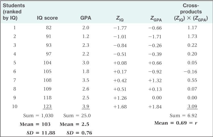
To continue the example described in Chapter 2, suppose you collected both the IQ score and GPA (grade-point average) for each of 10 different high school students and obtained the results shown in the “IQ score” and “GPA” columns of Table A.5. As a first step in determining the direction and strength of correlation between the two sets of scores, you might graph each pair of points in a scatter plot, as shown in Figure A.5 (compare this figure to Figure 2.3). The scatter plot makes it clear that, in general, the students with higher IQs tended to have higher GPAs, so you know that the correlation coefficient will be positive. However, the relationship between IQ and GPA is by no means perfect (the plot does not form a straight line), so you know that the correlation coefficient will be less than 1.00.
Calculation of a correlation coefficient (r)
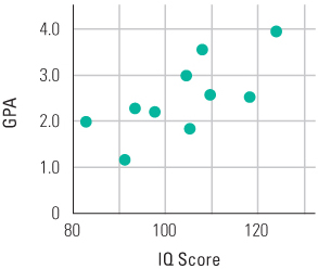
Each point represents the IQ and the GPA for 1 of the 10 students whose scores are shown in Table A.5. (For further explanation, refer to Figure 2.3 in Chapter 2.)
The first step in calculating a correlation coefficient is to convert each score to a z score, using the method described in the section on standardizing scores. Each z score, remember, is the number of standard deviations that the original score is away from the mean of the original scores. The standard deviation for the 10 IQ scores in Table A.5 is 11.88, so the z scores for IQ (shown in the column marked zIQ) were calculated by subtracting the mean IQ score (103) from each IQ and dividing by 11.88. The standard deviation for the ten GPA scores in Table A.5 is 0.76, so the z scores for GPA (shown in the column marked zGPA) were calculated by subtracting the mean GPA (2.5) from each GPA and dividing by 0.76.
To complete the calculation of the correlation coefficient, you multiply each pair of z scores together, obtaining what are called the z-score cross-products, and then determine the mean of those cross-products. The product-moment correlation coefficient, r, is, by definition, the mean of the z-score cross-products. In Table A.5, the z-score cross-products are shown in the right-hand column, and the mean of them is shown at the bottom of that column. As you can see, the correlation coefficient in this case is +0.69—a rather strong positive correlation.
A9