2.3 Statistical Methods in Psychology

To make sense of the data collected in a research study, we must have some way of summarizing the data and some way to determine the likelihood that observed patterns in the data are (or are not) simply the results of chance. The statistical procedures used for these purposes can be divided into two categories: (1) descriptive statistics, which are used to summarize sets of data, and (2) inferential statistics, which help researchers decide how confident they can be in judging that the results observed are not due to chance. We look briefly here at some commonly used descriptive statistics and then at the rationale behind inferential statistics. A more detailed discussion of some of these procedures, with examples, can be found in the Statistical Appendix at the back of this book.

Descriptive Statistics

Descriptive statistics include all numerical methods for summarizing a set of data. There are a number of relatively simple statistics that are commonly used to describe a set of data. These include the mean, median, and a measure of variability.

Describing a Set of Scores

If our data were a set of numerical measurements (such as ratings from 1 to 10 on how generous people were in their charitable giving), we might summarize these measurements by calculating either the mean or the median. The mean is simply the arithmetic average, determined by adding the scores and dividing the sum by the number of scores. The median is the center score, determined by ranking the scores from highest to lowest and finding the score that has the same number of scores above it as below it, that is, the score representing the 50th percentile. (The Statistical Appendix explains when the mean or the median is the more appropriate statistic.)

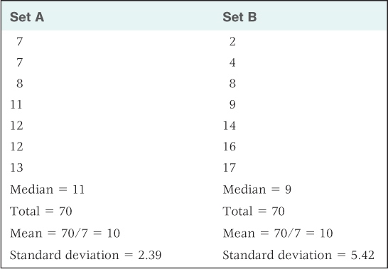
For certain kinds of comparisons, researchers need to describe not only the central tendency (the mean or median) but also the variability of a set of numbers. Variability refers to the degree to which the numbers in the set differ from one another and from their mean. In Table 2.1 you can see two sets of numbers that have identical means but different variabilities. In set A, the scores cluster close to the mean (low variability); in set B, they differ widely from the mean (high variability). A common measure of variability is the standard deviation, which is calculated by a formula described in the Statistical Appendix. As illustrated in Table 2.1, the further most individual scores are from the mean, the greater is the standard deviation.

Table 2-1: Table 2.1
Two sets of data, with the same mean but different amounts of variability

Describing a Correlation

Correlational studies, as discussed earlier in this chapter, examine two or more variables to determine whether or not a nonrandom relationship exists between them. When both variables are measured numerically, the strength and direction of the relationship can be assessed by a statistic called the correlation coefficient. Correlation coefficients are calculated by a formula (described in the Statistical Appendix) that produces a result ranging from −1.00 to +1.00. The sign (+ or −) indicates the direction of the correlation (positive or negative). In a positive correlation, an increase in one variable coincides with a tendency for the other variable to increase; in a negative correlation, an increase in one variable coincides with a tendency for the other variable to decrease. The absolute value of the correlation coefficient (the value with sign removed) indicates the strength of the correlation. To the degree that a correlation is strong (close to +1.00 or −1.00), you can predict the value of one variable by knowing the other. A correlation close to zero (0) means that the two variables are statistically unrelated—knowing the value of one variable does not help you predict the value of the other.

As an example, consider a hypothetical research study conducted with 10 students in a college course, aimed at assessing the correlation between the students’ most recent test score and each of four other variables: (1) the hours they spent studying for the test; (2) the score they got on the previous test; (3) their level of psychological depression, measured a day before the test; and (4) their height in centimeters. Suppose the data collected in the study are those depicted in the table on the next page in Figure 2.3. Each row in the table shows the data for a different student, and the students are rank ordered in accordance with their scores on the test.

Figure 2-3: Examples of correlations, using made-up data The table above shows the most recent test score and four other measures for each of 10 students in a college course. At the bottom of each of the four right-hand columns is the correlation coefficient relating the data of that column to the test score. (The study is fictitious and the data were made up for illustrative purposes.) The four scatter plots depict, separately, the correlation between the test score and each of the four other measures. By comparing the plots, you can see the difference between weaker and stronger correlations and between positive and negative correlations.

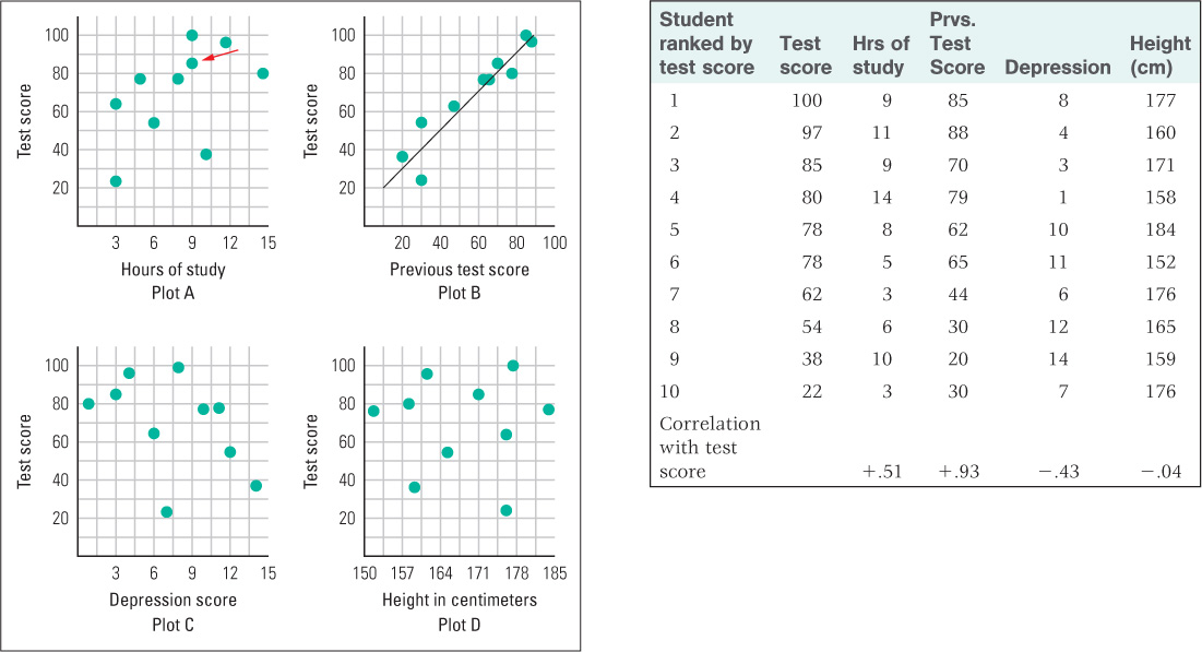
To visualize the relationship between the test score and any of the other four variables, the researcher might produce a scatter plot, in which each student’s test score and that student’s value for one of the other measurements are designated by a single point on the graph. The scatter plots relating test score to each of the other variables are shown in Figure 2.3:

• Plot A illustrates the relation between test score and hours of study. Notice that each point represents both the test score and the hours of study for a single student. Thus, the point indicated by the red arrow denotes a student whose score is 85 and who spent 9 hours studying. By looking at the whole constellation of points, you can see that, in general, higher test scores correspond with more hours spent studying. This is what makes the correlation positive. But the correlation is far from perfect. It can be described as a moderate positive correlation. (The calculated correlation coefficient is +.51.)
• Plot B, which relates this test score to the score on the previous test, illustrates a strong positive correlation. Notice that in this plot the points fall very close to an upwardly slanted line. The closer the points are to forming a straight line, the stronger is the correlation between the two variables. In this study, score on the previous test is an excellent predictor of the score on the new test. (The correlation coefficient is +.93.)

• Plot C, which shows the relation between test score and depression, illustrates a moderate negative correlation. Test score tends to decrease as depression increases. (The correlation coefficient here is −.43.)
• Plot D, which shows the relation between test score and height, illustrates uncorrelated data—a correlation coefficient close to or equal to 0. Knowing a person’s height provides no help in predicting the person’s test score. (The correlation coefficient here is −.04.)

Inferential Statistics

Any set of data collected in a research study contains some degree of variability that can be attributed to chance. That is the essential reason why inferential statistics are necessary. In the experiment comparing treatments for depression summarized back in Figure 2.1, the average depression scores obtained for the four groups reflect not just the effects of treatment but also random effects caused by uncontrollable variables. For example, more patients who were predisposed to improve could by chance have been assigned to one treatment group rather than to another. Or measurement error stemming from imperfections in the rating procedure could have contributed to differences in the depression scores. If the experiment were repeated several times, the results would be somewhat different each time because of such uncontrollable random variables. Given that results can vary as a result of chance, how confident can a researcher be in inferring a general conclusion from the study’s data? Inferential statistics are ways of answering that question using the laws of probability.

Statistical Significance

When two groups of subjects in an experiment have different mean scores, the difference might be meaningful, or it might be just the result of chance. Similarly, a nonzero correlation coefficient in a correlational study might indicate a meaningful relationship between two variables—or it might be just the result of chance, such as flipping a coin 10 times and coming up with heads on seven of them. Seven is more than you would expect from chance if it’s a fair coin (that would be five), but with only 10 tosses you could have been “just lucky” in getting seven heads. If you got heads on 70 out of 100 flips (or 700 out of 1,000), you’d be justified in thinking that the coin is not “fair.” Inferential statistical methods, applied to either an experiment or a correlational study, are procedures for calculating the probability that the observed results could derive from chance alone.

© The New Yorker Collection, Leo Cullen, from cartoonbank.com. All Rights Reserved.

Using such methods, researchers calculate a statistic referred to as p (for probability), or the level of significance. When two means are being compared, p is the probability that a difference as great as or greater than that observed would occur by chance if, in the larger population, there were no difference between the two means. (“Larger population” here means the entire set of scores that would be obtained if the experiment were repeated an infinite number of times with all possible subjects.) In other words, in the case of comparing two means in an experiment, p is the probability that a difference as large as or larger than that observed would occur if the independent variable had no real effect on the scores. In the case of a correlational study, p is the probability that a correlation coefficient as large as or larger than that observed (in absolute value) would occur by chance if, in the larger population, the two variables were truly uncorrelated. By convention, results are usually labeled as statistically significant if the value of p is less than .05(5 percent). To say that results are statistically significant is to say that the probability is acceptably small (generally less than 5 percent) that they could be caused by chance alone. All of the results of experiments and correlational studies discussed in this textbook are statistically significant at the .05 level or better.

The Components of a Test of Statistical Significance

The precise formulas used to calculate p values for various kinds of research studies are beyond the scope of this discussion, but it is worthwhile to think a bit about the elements that go into such calculations. They are:

1. The size of the observed effect. Other things being equal, a large effect is more likely to be significant than a small one. For example, the larger the difference found between the mean scores for one group compared to another in an experiment, or the larger the absolute value of the correlation coefficient in a correlational study, the more likely it is that the effect is statistically significant. A large effect is less likely to be caused just by chance than is a small one.
2. The number of individual subjects or observations in the study. Other things being equal, results are more likely to be significant the more subjects or observations included in a research study. Large samples of data are less distorted by chance than are small samples. The larger the sample, the more accurately an observed mean, or an observed correlation coefficient, reflects the true mean, or correlation coefficient, of the population from which it was drawn. If the number of subjects or observations is huge, then even very small effects will be statistically significant, that is, reflect a “true” difference in the population.
3. The variability of the data within each group. This element applies to cases in which group means are compared to one another and an index of variability, such as the standard deviation, can be calculated for each group. Variability can be thought of as an index of the degree to which uncontrolled, chance factors influence the scores in a set of data. For example, in the experiment assessing treatments for depression, greater variability in the depression scores within each treatment group would indicate greater randomness attributable to chance. Other things being equal, the less the variability within each group, the more likely the results are to be significant. If all of the scores within each group are close to the group mean, then even a small difference between the means of different groups may be significant.

In short, a large observed effect, a large number of observations, and a small degree of variability in scores within groups all reduce the likelihood that the effect is due to chance and increase the likelihood that a difference between two means, or a correlation between two variables, will be statistically significant.

Statistical significance tells us that a result probably did not come about by chance, but it does not, by itself, tell us that the result has practical value. Don’t confuse statistical significance with practical significance. If we were to test a new weight-loss drug in an experiment that compared 10,000 people taking the drug with a similar number not taking it, we might find a high degree of statistical significance even if the drug produced an average weight loss of only a few ounces. In that case, most people would agree that, despite the high statistical significance, the drug has no practical significance in a weight-loss program.