Thinking Under Uncertainty
We live in an uncertain world; everything that happens has a probability. For example, there is a probability for whether it will rain today and another probability for whether you will get an “A” in this class. The probability of an event is the likelihood that it will happen. Probabilities range from 0 (never happens) to 1 (always happens), but they are usually uncertain, somewhere between 0 and 1. An event with a probability of 0.5 is maximally uncertain because it is equally likely to occur and not to occur. Because we live in an uncertain world, we have to learn to estimate the probabilities (uncertainties) of various events. But how do we do this? Let’s try to estimate some probabilities.
239
Consider this: Does the letter r occur more often as the first letter or third letter in English words? To answer this question, you need to make a judgment about the probability of one event (r occurring as the first letter) in relation to the probability of a second event (r occurring as the third letter). Think about how you would estimate these probabilities. One way to proceed would be to compare the ease of thinking of words beginning with r versus having r in the third position. Isn’t it easier to think of words beginning with r? Does this mean that such words occur more often and that this event is more probable? If you think so, you are using a heuristic (words that are more available in our memory are more probable) to answer the probability question. When we discuss the main heuristics that humans use to judge probabilities, we’ll return to this problem and see if this heuristic led us to the correct answer.
In addition to judging the uncertainty of events in our environment, we attempt to reduce our uncertainty about the world by trying to find out how various events are related to each other. For example, is the amount of arthritis pain related to the weather? To answer such questions, we develop and test hypotheses about how the events in our world are related. Such hypothesis testing allows us to learn about the world. Many of our beliefs are the conclusions that we have arrived at from testing such hypotheses. However, we usually don’t test our hypotheses in well-controlled formal experiments the way that psychologists do. Instead we conduct subjective, informal tests of our hypotheses. Obviously, such a nonscientific approach may be biased and result in incorrect conclusions and erroneous beliefs. A good example is belief in the paranormal. If you are like most college students, you probably believe in at least one paranormal phenomenon, such as mental telepathy, clairvoyance, or psychokinesis (Messer & Griggs, 1989). But, as you learned in Chapter 3, there is not one replicable scientific finding for any of these phenomena. We’ll discuss how such erroneous beliefs might arise from our subjective hypothesis testing method.
We also often engage in hypothesis testing in various medical situations. One very common instance is testing the hypothesis that we have a specific disease given a positive result on a medical screening test for the disease. This actually amounts to trying to compute a conditional probability, which for most people (doctors and patients) is not that easy. Research that we will discuss shows that both doctors and patients tend to greatly overestimate such probabilities. To help you more accurately assess your chances of having the disease in this situation, we’ll teach you a relatively simple way to compute such probabilities. But first let’s see how we judge probabilities in general and how these judgments might be biased.
Judging Probability
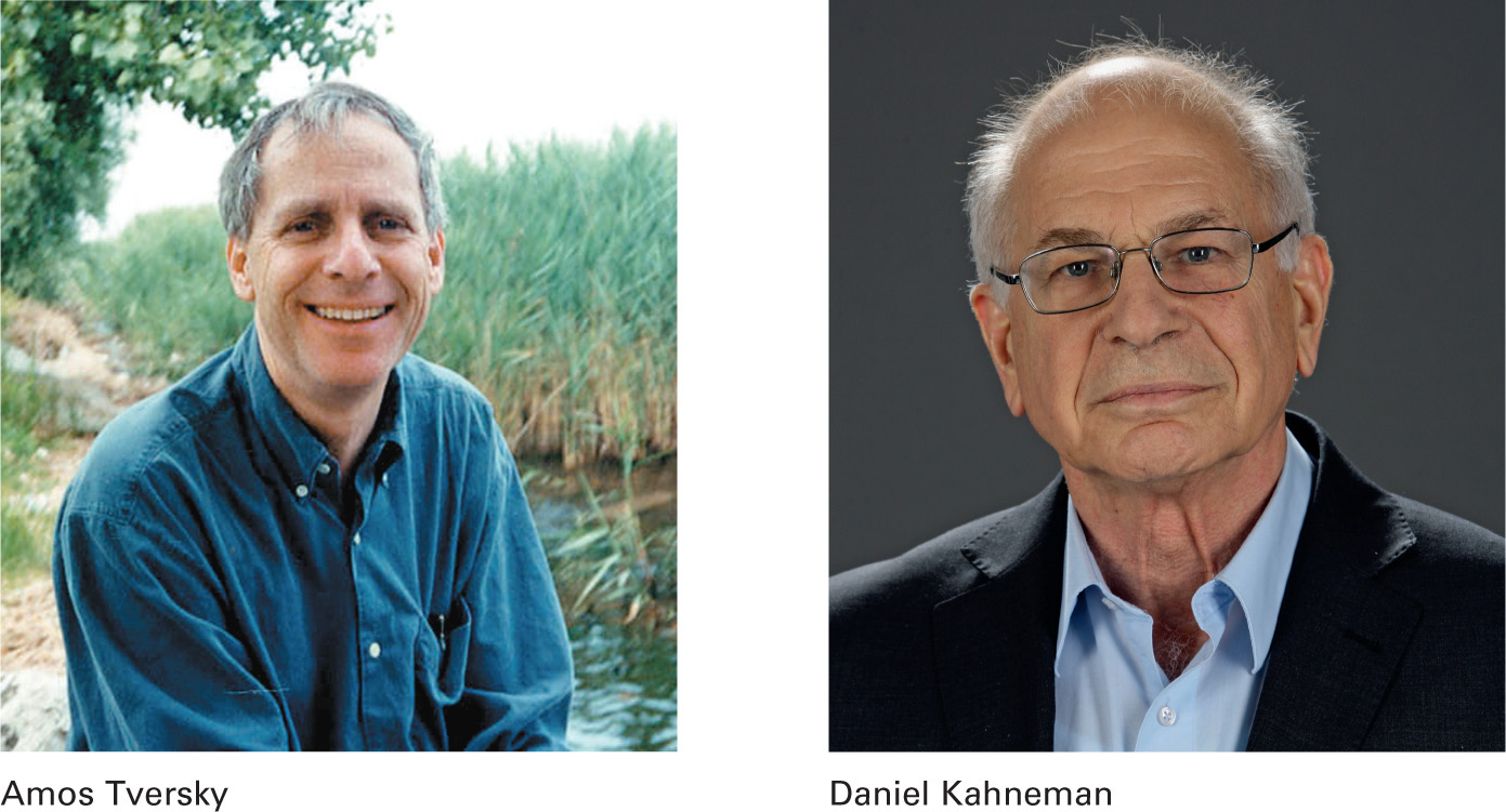
Cognitive psychologists Amos Tversky and Daniel Kahneman identified two heuristics that we often use to make judgments about probabilities—the representativeness heuristic and the availability heuristic (Tversky & Kahneman, 1974). It is important to point out that these two heuristics usually lead to reasonably good judgments, but they sometimes lead to errors. Why? The major reason is that a heuristic can lead us to ignore information that is extremely relevant to the particular probability judgment. To understand, let’s consider the following problem (Tversky & Kahneman, 1983).
240
Andreas Rentz/Getty Images for Burda Media
You will read a brief description of Linda, and then you will be asked to make a judgment about her. Here’s the description:
Linda is 31 years old, single, outspoken, and very bright. She majored in philosophy. As a student, she was deeply concerned with issues of discrimination and social justice, and also participated in antinuclear demonstrations.
Which of the following alternatives is more likely?
Linda is a bank teller.
Linda is a bank teller and active in the feminist movement.
The representativeness heuristic.
To decide which alternative is more probable, most people would use what is called the representativeness heuristic—a rule of thumb for judging the probability of membership in a category by how well an object resembles (is representative of) that category. Simply put, the rule is: the more representative, the more probable. Using this heuristic, most people, including undergraduates, graduate students, and professors, judge that the second alternative (Linda is a bank teller and active in the feminist movement) is more likely than the first alternative (Tversky & Kahneman, 1983). Why? Linda resembles someone active in the feminist movement more than she resembles a bank teller. However, it is impossible for the second alternative to be more likely than the first. Actually the description of Linda is totally irrelevant to the probability judgment!
241
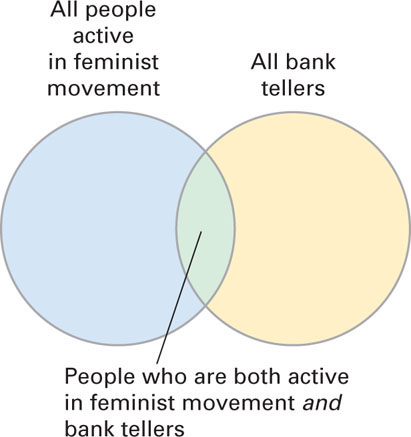
Let’s look at the set diagram in Figure 6.1. This diagram illustrates what is known as the conjunction rule for two different uncertain events (in this case, being a bank teller and being active in the feminist movement). The conjunction rule is that the likelihood of the overlap of two uncertain events (the green section of the diagram) cannot be greater than the likelihood of either of the two events because the overlap is only part of each event. This means that all of the tellers who are active in the feminist movement make up only part of the set of all bank tellers. Because the set of bank tellers is larger and includes those tellers who are active in the feminist movement, it is more likely that someone is a bank teller than that someone is a bank teller and active in the feminist movement. Judging that it is more likely that Linda is a bank teller and active in the feminist movement illustrates the conjunction fallacy—incorrectly judging the overlap of two uncertain events to be more likely than either of the two events. By using the representativeness heuristic, we overlook a very simple principle of probability, the conjunction rule. This illustrates the shortcoming of using such heuristics—overlooking essential information for making the probability judgment.
Using the representativeness heuristic also leads to the gambler's fallacy—the erroneous belief that a chance process is self-correcting in that an event that has not occurred for a while is more likely to occur. Suppose a person has flipped eight heads in a row and we want to bet $100 on the next coin toss, heads or tails. Some people will want to bet on tails because they think it more likely, but in actuality the two events are still equally likely. One of the most famous examples of the gambler’s fallacy occurred in a Monte Carlo casino in 1913 when a roulette wheel landed on black 26 times in a row (Lehrer, 2009). During that run, most people bet against black since they felt that red must be “due.” They assumed that the roulette wheel would somehow correct the imbalance and cause the wheel to land on red. The casino ended up making millions of francs. “The wheel has no mind, no soul, no sense of fairness…Yet, we often treat it otherwise” (Vyse, 1997, p. 98).
242
Why do people commit the gambler’s fallacy? Again, they are using the representativeness heuristic (Tversky & Kahneman, 1971). People believe that short sequences (the series of eight coin tosses or the 26 spins of the roulette wheel) should reflect the long-run probabilities. Simply put, people believe random sequences, whether short or long, should look random. This is not the case. Probability and the law of averages only hold in the long run, not the short run. In addition, the long run is indeed very long—infinity. The representativeness heuristic leads us to forget this.
Why are we so prone to using the representativeness heuristic and making judgments based only on categorical resemblance? The answer is tied to the fact that the mind categorizes information automatically. Categorization is just another name for pattern recognition, an automatic process that we discussed in Chapter 3. The brain constantly recognizes (puts into categories) the objects, events, and people in our world. Categorization is one of the brain’s basic operational principles, so it shouldn’t be surprising that we may judge categorical probabilities in the same way that we recognize patterns. This is how the brain normally operates. In addition to probability judgments, the representativeness heuristic can lead us astray in judging the people we meet because our first impression is often based on categorical resemblance. We tend to categorize the person based on the little information we get when we meet him or her. Remember that this initial judgment is only an anchor, and we need to process subsequent information carefully in order to avoid misjudgment of the person.
The availability heuristic.
Let’s go back to the judgment that you made earlier. Does the letter r appear more often as the first letter or third letter in English words? Actually, the letter r appears twice as often as the third letter in words than as the first letter. However, if you used the availability heuristic that was described, you would judge the reverse to be the case (that r occurs more often as the first letter). The availability heuristic is the rule of thumb that the more available an event is in our memory, the more probable it is (Tversky & Kahneman, 1973). We can think of more words beginning with the letter r than with r in the third position because we organize words in our memories by how they begin. This does not mean that they are more frequent, but only that it is easier to think of them. They are easier to generate from memory. The opposite is the case—words with r in the third position are more frequent. This is actually true for seven letters: k, l, n, r, v, x, and z (Tversky & Kahneman, 1973).
Remember that a heuristic does not guarantee a correct answer. The availability heuristic may often lead to a correct answer; but as in the letter r problem, events are sometimes more easily available in our memories for reasons other than how often they actually occur. An event may be prominent in our memories because it recently happened or because it is particularly striking or vivid. In such cases, the availability heuristic will lead to an error in judgment. Think about judging the risk of various causes of death. Some causes of death (airplane crashes, fires, and shark attacks) are highly publicized and thus more available in our memories, especially if they have occurred recently. Using the availability heuristic, we judge them to be more likely than lesser publicized, less dramatic causes of death such as diabetes and emphysema, which are actually more likely but not very available in our memories (Lichtenstein, Slovic, Fischhoff, Layman, & Combs, 1978). In fact, the probability of dying from falling airplane parts is 30 times greater than that of being killed by a shark (Plous, 1993). The lesson to be learned here is that greater availability in memory does not always equal greater probability.
243

Availability in memory also plays a key role in what is termed a dread risk. A dread risk is a low-probability, high-damage event in which many people are killed at one point in time. Not only is there direct damage in the event, but there is secondary, indirect damage mediated through how we psychologically react to the event. A good example is our reaction to the September 11, 2001, terrorist attacks (Gigerenzer, 2004, 2006). Fearing dying in a terrorist airplane crash because the September 11 events were so prominent in our memories, we reduced our air travel and increased our automobile travel, leading to a significantly greater number of fatal traffic accidents than usual. It is estimated that about 1,600 more people needlessly died in these traffic accidents (Gigerenzer, 2006). These lives could have been saved had we not reacted to the dread risk as we did. We just do not seem to realize that it is far safer to fly than to drive. National Safety Council data reveal that you are 37 times more likely to die in a vehicle accident than on a commercial flight (Myers, 2001).
Since heuristics may mislead us, you may wonder why we rely upon them so often. First, heuristics are adaptive and often serve us well and lead to a correct judgment. Second, they stem from what cognitive psychologists call System 1 (automatic) processing (Evans, 2008, 2010; Stanovich & West, 2000). System 1 processing is part of a dual processing system and is contrasted with System 2 (reflective) processing. Kahneman (2011) refers to System 1 as fast, intuitive, and largely unconscious thinking and System 2 as slow, analytical, and consciously effortful thinking. Although System 2 is responsible for more rational processing and can override System 1, it is also lazy. System 2 is willing to accept the easy but possibly unreliable System 1 answer. Clearly there are shortcomings with the System 1 heuristics that we use to judge probabilities (uncertainties). Thus, you should work to engage System 2 processing. Slow down your thinking; be more analytical. For example, make sure you have not overlooked relevant probability information when using the representativeness heuristic, and try to think beyond prominence in memory when using the availability heuristic. In brief, don’t “rush to judgment.” Are there also shortcomings with the way we try to reduce our uncertainty and learn about the world through hypothesis testing? We now turn to this question.
244
Hypothesis Testing
In Chapter 1, we discussed the experimental research method that psychologists use to test their hypotheses about human behavior and mental processing. Like psychologists, we too have beliefs about the relationships between the variables in our environment (hypotheses), and we too collect data to test these beliefs. However, we don’t use the experimental method discussed in Chapter 1. So what do we do? How do people test their hypotheses and thus reduce their uncertainty about the world? British researcher Peter Wason devised two problems to examine this question—the 2-4-6 task and the four-card selection task.
Confirmation bias.
In the 2-4-6 task, you are presented the number sequence “2-4-6” and asked to name the rule that the experimenter used to generate that sequence (Wason, 1960). Before presenting your hypothesized rule (your answer), you are allowed to generate as many sequences of three numbers as you want and get feedback on whether each conforms to the experimenter’s rule. When you think that you know the rule, you tell the experimenter. Before we describe how people perform on this task, think about how you would proceed. What would be your first hypothesis for the rule and what sequences of three numbers would you generate to test your hypothesized rule?
245
Most of the participants do not name the correct rule. They devise a hypothesis (e.g., “numbers increasing by 2”) and proceed to test the hypothesis by generating series that conform to it (e.g., 8-10-12). In other words, they test their hypotheses by trying to confirm them. Did you do this? People do not test their hypotheses by trying to disconfirm them (e.g., generating the sequence 10-11-12 for the hypothesis “numbers increasing by 2”). The tendency to seek evidence that confirms one’s beliefs is called confirmation bias. This bias is pervasive in our everyday hypothesis testing, so it is not surprising that it occurs on the 2-4-6 task. The 2-4-6 task serves to highlight the inadequacy of the confirmation bias as a way to test a hypothesis. To truly test a hypothesis, we must try to disconfirm it. We should attempt to disconfirm each hypothesis that we generate. The experimenter’s rule for the 2-4-6 task was a very simple, general rule, so most sequences that people generated conformed to it. What was it? The rule was simply any three increasing numbers; how far apart the numbers were did not matter.
Now let’s look at the four-card selection task (Wason, 1966, 1968). Try the problem before reading further.
The four cards below have information on both sides. On one side of a card is a letter, and on the other side is a number.
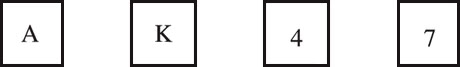
Consider this rule: If a card has a vowel on one side, then it has an even number on the other side.
Select the card or cards that you definitely must turn over to determine whether the rule is true or false for these four cards.
Well, if you’re like most people, you haven’t answered correctly. The correct response rate for this problem is usually less than 10 percent (Griggs & Cox, 1982). The most frequent error is to select the cards showing A and 4. The card showing A is part of the correct solution, but the card showing 4 is not. You should select the cards showing A and 7. Why? First, you should decide what type of card would falsify the rule. The rule states that if a card has a vowel on one side, it has to have an even number on the other side. Therefore, a card with a vowel on one side and an odd number on the other side would falsify the rule. Now do you see why the answer is A and 7? An odd number on the other side of the A card would falsify the rule, and so would a vowel on the other side of the 7 card. No matter what is on the other side of the K and 4 cards, the rule is true.
So why do people select the cards showing A and 4? As in the 2-4-6 task, people focus on confirmation and select cards to verify the rule (show that it is true). They choose the cards showing A and 4 because they incorrectly think that the rule must hold in both directions (it doesn’t) and they must verify that it does so. They choose the card showing a vowel (A) to verify that it has an even number on the other side and the card showing an even number (4) to verify that it has a vowel on the other side. Instead of deducing what will falsify (disconfirm) the rule, people merely try to confirm it (demonstrating confirmation bias). There is, however, some recent evidence that people motivated to reject a rule because it is personally threatening or disagreeable to them will focus on disconfirmation and thus perform better on the four-card selection task (Dawson, Gilovich, & Regan, 2002).
246
Research on the 2-4-6 task and the four-card selection task show that people typically try to confirm hypotheses. Confirmation bias, however, is not limited to the 2-4-6 and four-card selection tasks, but extends to many aspects of our daily lives such as jury decisions, physicians’ diagnoses, and the justification of governmental policies (Nickerson, 1998). In addition, it leads to other cognitive difficulties. For example, confirmation bias may lead us to perceive illusory correlations between events in our environment (Chapman, 1967; Chapman & Chapman, 1967). An illusory correlation is the erroneous belief that two variables are statistically related when they actually are not. If we believe a relationship exists between two things, then we will tend to notice and remember instances that confirm this relationship. Let’s consider an example.
Many people erroneously believe that a relationship exists between weather changes and arthritis. Why? They focus on instances when the weather changes and their arthritic pain increases. To determine if this relationship actually exists, we need to consider the frequency of all four possible events, the two that confirm the hypothesis and the two that disconfirm it. In our example, the two confirming instances would be (1) when the weather changes and arthritic pain changes, and (2) when the weather does not change and arthritic pain does not change. The two disconfirming instances are (1) when the weather changes but arthritic pain does not, and (2) when the weather does not change but arthritic pain does. When the frequencies of all four events are considered, it turns out that there isn’t a relationship between these two variables. The confirming events are not more frequent than the disconfirming events (Redelmeier & Tversky, 1996).
Confirmation bias is likely responsible for many of our erroneous beliefs. Science provides better answers than informal, biased hypothesis testing. When our beliefs are contradicted by science, as in the case of belief in paranormal events, we should think about our hypothesis testing procedure versus that of the scientist. We may have only gathered evidence to support our belief. We have to be willing to accept that our beliefs may be wrong. This is not easy for us to do. We suffer from belief perseverance—the tendency to cling to our beliefs in the face of contradictory evidence (Anderson, Lepper, & Ross, 1980). Our beliefs constitute a large part of our identity; therefore, admitting that we are wrong is very difficult. Such denial is illustrated by person-who reasoning—questioning a well-established finding because we know a person who violates the finding (Nisbett & Ross, 1980; Stanovich, 2004). A good example is questioning the validity of the finding that smoking leads to health problems, because we know someone who has smoked most of his or her life and has no health problems. Such reasoning also likely indicates a failure to understand that these research findings are probabilities. Such research findings are not certain; they do not hold in absolutely every case. Exceptions to these sorts of research findings are to be expected. Person-who reasoning is not valid, and we shouldn’t engage in it.
247
Testing medical hypotheses.
As we pointed out, confirmation bias seems to impact physicians’ testing of hypotheses during the diagnostic process (Nickerson, 1998). Physicians (and patients) also seem to have difficulty in interpreting positive test results for medical screening tests, such as for various types of cancer and HIV/AIDS (Gigerenzer, 2002). They often overestimate the probability that a patient has a disease based on a positive test result. When considering what a positive result for a screening test means, you are testing the hypothesis that a patient actually has the disease being screened for by determining the probability that the patient has the disease given a positive test result. Because you will be considering the results of medical screening tests throughout your lifetime and will inevitably get some positive results, you should understand how to compute this conditional probability in order to know your chances of actually having the disease. Because this computation is not a very intuitive process, I will show you a straightforward way to do it, so that you can make more informed medical decisions.
Much of the research that is focused on how successful doctors and patients are at correctly interpreting a positive result for a medical screening test and on how they can improve their performance has been conducted by Gerd Gigerenzer and his colleagues (Gigerenzer, 2002; Gigerenzer & Edwards, 2003; Gigerenzer, Gaissmaier, Kurz-Milcke, Schwartz, & Woloshin, 2007). Both doctors and patients have been found to overestimate these conditional probabilities. An older study by Eddy (1982) with 100 American doctors as the participants illustrates this overestimation finding; but before considering it, some explanation is necessary. In medicine, probabilities are often expressed in percentages rather than as numbers between 0 and 1.0. Three terms relevant to screening tests, the base rate for a disease and the sensitivity and false positive rates for the test, also need to be explained before we continue. The base rate (prevalence) of a disease is simply the probability with which it occurs in the population. The sensitivity rate for a screening test is the probability that a patient tests positive if she has the disease, and the false positive rate is the probability that a patient tests positive if she does not have the disease. Now consider Eddy’s problem. You should try to estimate the probability asked for in the problem before reading on.
248
- Estimate the probability that a woman has breast cancer given a positive mammogram result and a base rate for this type of cancer of 1%, a sensitivity rate for the test of 80%, and a false positive rate for the test of 9.6%.
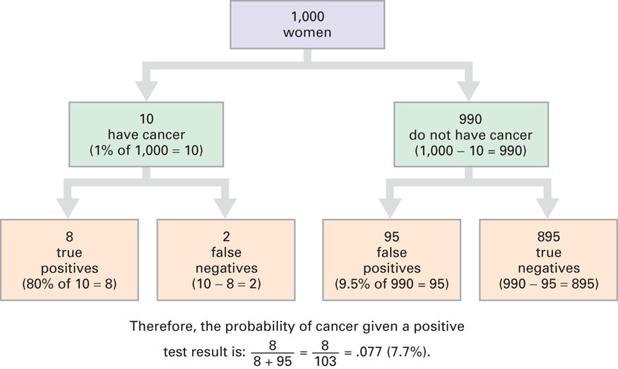
What was your estimate? If you acted like the doctors, you overestimated the probability. Almost all of the doctors estimated this probability to be around 75 percent. The correct answer, however, is much less, only around 8 percent. Hoffrage and Gigerenzer (1998) replicated Eddy’s finding with even more shocking results. Physicians’ estimates ranged from 1 percent to 90 percent, with a 90 percent chance of breast cancer being the most frequent estimate. Given the doctors’ overestimation errors, think of how many women who tested positive in this case would have been unnecessarily alarmed had this been real life and not an experiment. Think about the possible consequences, which are far from trivial—emotional distress, further testing, biopsy, more expense, and maybe even unnecessary surgery. To correctly compute the conditional probability that someone has the disease given a positive test result, Gigerenzer recommends that you convert all of the percentages (probabilities) into natural frequencies, or simple counts of events. According to Gigerenzer, natural frequencies represent the way humans encoded information before probabilities were invented and are easier for our brains to understand. In brief, they make more sense to us. To convert to natural frequencies, we begin by supposing there is a sample of women who have had the screening test. It’s best to suppose a large, even number such as 1,000, because such numbers allow an easier conversion to natural frequencies. Assuming a sample of 1,000 women, we can then proceed to convert Eddy’s percentages into natural frequencies and compute the conditional probability.
Given a base rate of 1%, we would expect 10 (1% of 1,000) women to have breast cancer.
Of these 10, we expect 8 (80% of 10) to test positive because the test has a sensitivity rate of 80%. The results for these 8 women are called true positives because these women have breast cancer and their test results were positive. The test results for the other 2 women are called false negatives because these women have breast cancer but their test results were negative.
Among the 990 (1,000 − 10) women without breast cancer, 95 (9.6% of 990) will test positive given the 9.6% false positive rate. The results for these 95 women are called false positives because these women do not have cancer but their test results were positive. The results for the remaining 895 women are called true negatives because these women do not have cancer and their test results were negative.
Thus, 103 (8 + 95) women in the sample of 1,000 will test positive, but only 8 are true positives. Thus, the conditional probability that a woman testing positive actually has cancer is the percentage of positive test results that are true positives, 8/103 = 0.077 (7.7%).
Hoffrage and Gigerenzer (1995) found that once they presented the numbers as natural frequencies to doctors, the majority suddenly understood the problem. Do you? If not, the solution steps are visually illustrated in the natural frequency tree diagram in Figure 6.2. Read through the steps in the tree diagram and then read through them again in the text. After doing this, you should better understand how to do such calculations.
249
It should be clear to you now that a positive result for a medical screening test does not necessarily mean that you have the disease. You might or you might not. It is natural to assume the worst when faced with a positive test result, but it may be more probable that you do not have the disease. There is uncertainty, and the hypothesis that you have the disease must be tested by computing the conditional probability that you do, given the positive test result. You now know how to do this by representing the base, sensitivity, and false positive rates as natural frequencies and using these frequencies to compute the probability. Combine a low incidence rate (for example, 1 or 2 percent) with just a modest false positive rate (for example, 10 percent) for a screening test, and there will be many false positives (Mlodinow, 2008). A good example is mammography with young women. In this case, a positive mammogram is actually more likely not to indicate cancer. Of course, screening tests with high false positive rates are also problematic, leading to both overdiagnosis and overtreatment. A good example is the PSA test for prostate cancer in men (Gilligan, 2009). Given that the potential benefits do not outweigh the harms for this test, the U.S. Preventive Services Task Force (the federal panel empowered to evaluate cancer screening tests) recommended in 2012 against PSA screening for men, regardless of age (Moyer, 2012). For more detailed coverage of interpreting screening test results and understanding other medical statistics, see Gigerenzer (2002) and Woloshin, Schwartz, and Welch (2008).
250
Section Summary
In this section, we learned that when we make probability judgments, we often use the representativeness and availability heuristics. When using the representativeness heuristic, we judge the likelihood of category membership by how well an object resembles a category (the more representative, the more probable). This heuristic can lead us to ignore extremely relevant probability information such as the conjunction rule. The availability heuristic leads us to judge the likelihood of an event by its availability in memory (the more available, the more probable). We may make errors with the availability heuristic, because events may be highly prominent in our memories because of their recent occurrence or because they are particularly vivid and not because they occur more often. Using these heuristics arises from System 1 (automatic, intuitive) processing. We need to slow down our thinking and engage System 2 (effortful, analytical) processing to improve our judgment.
We also considered that when we test hypotheses about our beliefs, we tend to suffer from confirmation bias (the tendency to seek evidence that confirms our beliefs). This bias may lead us to have erroneous beliefs based on illusory correlations, believing two variables are related when they actually are not. To prevent this, we should attempt to disconfirm our hypotheses and beliefs rather than confirm them. Even in the face of contradictory evidence, we tend to persevere in our beliefs and ignore the evidence, or we engage in denial through invalid person-who statistical reasoning (thinking that a well-established finding should not be accepted because there are some exceptions to it). Lastly, we discussed medical hypothesis testing, specifically how to compute the conditional probability that a person actually has a disease that is being screened for, given a positive test result. Research indicates that both doctors and patients tend to overestimate such probabilities. The conversion of the relevant probability information, however, to natural frequencies greatly facilitates the computation of these conditional probabilities.
ConceptCheck | 2
 Explain how using the representativeness heuristic can lead to the conjunction fallacy.
The representativeness heuristic can lead to the conjunction fallacy by causing us to ignore the conjunction rule when making a probability judgment involving the conjunction of two uncertain events. Use of the heuristic for the Linda problem illustrates how this occurs. We focus on how much Linda resembles a feminist and ignore the conjunction rule that says that the probability that Linda is a bank teller has to be more probable than the conjunction of her being a bank teller and active in the feminist movement.
-
Explain how using the availability heuristic can lead to the misjudgment of the probabilities of various causes of death.
The availability heuristic can lead us to overestimate the risk of causes of death that are highly publicized (such as airplane crashes, fires, and shark attacks) and underestimate those that are less publicized and not as dramatic (such as diabetes and emphysema). Because the highly publicized causes are more available in our memories, we misjudge them to be more probable than the less publicized causes.
-
Explain how confirmation bias can lead to the perception of an illusory correlation.
Confirmation bias can lead to the perception of an illusory correlation by leading us to confirm our belief about the correlation by focusing only on events that confirm the belief and not on those that disconfirm the belief. To test to see if a relationship exists, we must consider the probabilities of both types of events.
-
Given a base rate of 2% for a disease and a false positive rate of 10% and a sensitivity rate of 90% for the screening test for the disease, use natural frequencies to compute the conditional probability that a person actually has the disease given a positive test result.
Assume that 1,000 people are screened for the disease. Given a base rate of 2% for the disease, only 20 (2% of 1,000) would actually have the disease. This means that 980 people (1,000 - 20) would not have the disease. Given a test sensitivity rate of 90%, 18 of the 20 (90% of 20) people who have the disease would test positive. Given a false positive rate of 10%, 98 (10% of 980) people who do not have the disease would test positive. Thus, there would be 116 positives (18 true positives and 98 false positives). Hence the conditional probability that someone testing positive actually has the disease is 18/116, which is 0.155 (15.5%).
251