28

Once we have completed an experiment, we need to understand our results and to describe them concisely so that others can understand them. To do this, we need to use statistics. There are two types of statistics—descriptive and inferential. We described inferential statistics when we discussed how to interpret the results of experimental studies. In this section, we will be discussing descriptive statistics—statistics used to describe the data of a research study in a concise fashion. The correlation coefficient that we discussed earlier is a descriptive statistic that allows us to describe the results of a correlational study precisely. For experimental findings, we need two types of descriptive statistics to summarize our data—measures of central tendency and measures of variability. In addition, a researcher often constructs a frequency distribution for the data. A frequency distribution depicts, in a table or a graph, the number of participants receiving each score for a variable. The bell curve, or normal distribution, is the most famous frequency distribution. We begin with the two types of descriptive statistics necessary to describe a data set: measures of central tendency and measures of variability.

In an experiment, the data set consists of the measured scores on the dependent variable for the sample of participants. A listing of this set of scores, or any set of numbers, is referred to as a distribution of scores, or a distribution of numbers. To describe such distributions in a concise summary manner, we use two types of descriptive statistics: measures of central tendency and measures of variability.

Measures of central tendency. The measures of central tendency define a “typical” score for a distribution of scores. There are three measures of central tendency (three ways to define the “typical” score)—mean, median, and mode. The first, the mean, is one that you are already familiar with from our earlier discussion of the regression toward the mean phenomenon. Remember, the mean is the numerical average for a distribution of scores. To compute the mean, you merely add up all of the scores and divide by the number of scores. A second measure of central tendency is the median—the score positioned in the middle of the distribution of scores when all of the scores are listed from the lowest to the highest. If there is an odd number of scores, the median is the middle score. If there is an even number of scores, the median is the halfway point between the two center scores. The final measure of central tendency, the mode, is the most frequently occurring score in a distribution of scores. Sometimes there are two or more scores that occur most frequently. In these cases, the distribution has multiple modes. Now let’s consider a small set of scores to see how these measures are computed.

29

Let’s imagine a class with five students who just took an exam. That gives us a distribution of five test scores: 70, 80, 80, 85, and 85. First, let’s compute the mean or average score. The sum of all five scores is 400. Now divide 400 by 5, and you get the mean, 80. What’s the median? It’s the middle score when the scores are arranged in ascending order. Because there is an odd number of scores (5), it’s the third score—80. If there had been an even number of scores, the median would be the halfway point between the center two scores. For example, if there had been only four scores in our sample distribution (70, 80, 85, and 85), the median would be the halfway point between 80 and 85, 82.5. Now, what’s the mode or most frequently occurring score? For the distribution of five scores, there are two numbers that occur twice, so there are two modes—80 and 85. This kind of distribution is referred to as a bimodal distribution (a distribution with two modes). Remember that a distribution can have one or more than one mode.

Of the three measures of central tendency, the mean is the one that is most commonly used. This is mainly because it is used to analyze the data in many inferential statistical tests. The mean can be distorted, however, by a small set of unusually high or low scores. In this case, the median, which is not distorted by such scores, should be used. To understand how atypical scores can distort the mean, let’s consider changing one score in our sample distribution of five scores. Change 70 to 20. Now, the mean is 70 (350/5). The median remains 80, however; it hasn’t changed. This is because the median is only a positional score. The mean is distorted because it has to average in the value of any unusual scores.

Measures of variability. In addition to knowing the typical score for a distribution, you need to determine the variability between the scores. For example, two distributions might have the same mean, but one distribution might have little variability between scores and the other, considerable variability between scores. So how is such variability measured? There are two measures of variability—the range and the standard deviation. The range is the simpler to compute. The range is simply the difference between the highest and lowest scores in the distribution. For our sample distribution with five scores, it would be 85 minus 70, or 15. However, like the mean, unusually high or low scores distort the range. For example, if the 70 in the distribution had been a 20, the range would change to be 85 minus 20, or 65. This would not be a good measure of the distribution’s variability because four of the five scores are 80 or 85, not very different.

The measure of variability used most often is the standard deviation. In general terms, the standard deviation is the average extent that the scores vary from the mean of the distribution. In other words, how spread out are the scores? If the scores do not vary much from the mean, the standard deviation will be small. If they vary a lot from the mean, the standard deviation will be larger. In our example of five test scores with a mean of 80, the scores (70, 80, 80, 85, and 85) didn’t vary much from this mean, therefore the standard deviation would not be very large. However, if the scores had been 20, 40, 80, 120, and 140, the mean would still be 80; but the scores vary more from the mean, therefore the standard deviation would be much larger.

30

The standard deviation and the various other descriptive statistics that we have discussed are summarized in Table 1.4. Review this table to make sure you understand each statistic. The standard deviation is especially relevant to the normal distribution, or bell curve. We will see in Chapter 6, on thinking and intelligence, that intelligence test scores are actually determined with respect to standard deviation units in the normal distribution. Next we will consider the normal distribution and the two types of skewed frequency distributions.

A frequency distribution organizes the data in a score distribution so that we know the frequency of each score. It tells us how often each score occurred. These frequencies can be presented in a table or visually in a figure. We’ll consider visual depictions. For many human traits (such as height, weight, and intelligence), the frequency distribution takes on the shape of a bell curve. For example, the heights of American adult men are distributed in a bell-shaped manner around a mean of 5 feet 10 inches (Wheelan, 2013). In fact, if a large number of people are measured on almost anything, the frequency distribution will visually approximate a bell-shaped curve. Statisticians call this bell-shaped frequency distribution, shown in Figure 1.3, the normal distribution.

31

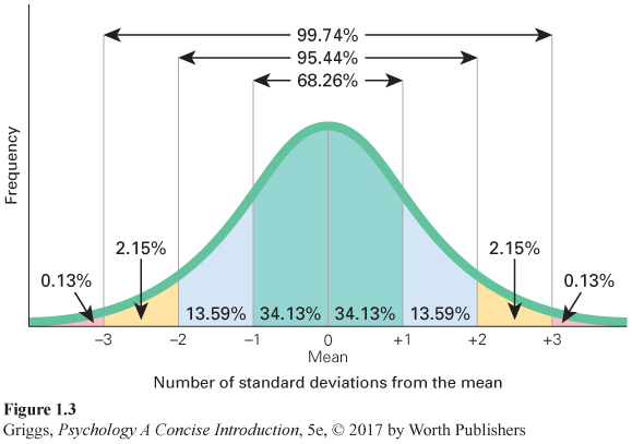
Normal distributions. There are two main aspects of a normal distribution. First, the mean, the median, and the mode are all equal because the normal distribution is symmetric about its center. You do not have to worry about which measure of central tendency to use because all of them are equal. The same number of scores fall below the center point as above it. Second, the percentage of scores falling within a certain number of standard deviations of the mean is set. About 68% of the scores fall within 1 standard deviation of the mean; about 95% within 2 standard deviations of the mean; and over 99% within 3 standard deviations of the mean. So what does this mean for the normal distribution of the heights of American adult men with a mean of 5 feet 10 inches? First, we have to know the standard deviation for this distribution. It is 3 inches. Thus, 68% of the heights of American men fall between 5 feet 7 inches (5 feet 10 inches – 3 inches) and 6 feet 1 inches (5 feet 10 inches + 3 inches), 95% between 5 feet 4 inches (5 feet 10 inches – 6 inches) and 6 feet 4 inches (5 feet 10 inches + 6 inches), and 99% between 5 feet 1 inch (5 feet 10 inches – 9 inches) and 6 feet 7 inches (5 feet 10 inches + 9 inches).

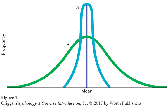
These percentages falling within a certain number of standard deviations are what give the normal distribution its bell shape. The percentages hold regardless of the size of the standard deviation for a normal distribution. Figure 1.4 shows two normal distributions with the same mean but different standard deviations. Both have bell shapes, but the distribution with the smaller standard deviation (A) is taller. As the size of the standard deviation increases, the bell shape becomes shorter and wider (like B).

32

The percentages of scores and the number of standard deviations from the mean always have the same relationship in a normal distribution. This allows you to compute percentile ranks for scores. A percentile rank is the percentage of scores below a specific score in a distribution of scores. If you know how many standard deviation units a specific score is above or below the mean in a normal distribution, you can compute that score’s percentile rank. For example, the percentile rank of a score that is 1 standard deviation above the mean is roughly 84%. Remember, a normal distribution is symmetric about the mean so that 50% of the scores are above the mean and 50% are below the mean. This means that the percentile rank of a score that is 1 standard deviation above the mean is greater than 50% (the percent below the mean) + 34% (the percent of scores from the mean to +1 standard deviation).

Now I’ll let you try to compute a percentile rank. What is the percentile rank for a score that is 1 standard deviation below the mean? Remember that it is the percentage of the scores below that score. Look at Figure 1.3. What percentage of the scores is less than a score that is 1 standard deviation below the mean? The answer is about 16%. You can never have a percentile rank of 100% because you cannot outscore yourself, but you can have a percentile rank of 0% if you have the lowest score in the distribution. The scores on intelligence tests and the SAT are based on normal distributions, so percentile ranks can be calculated for these scores. We will return to the normal distribution when we discuss intelligence test scores in Chapter 6.

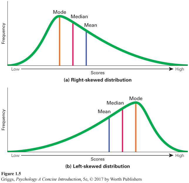
Skewed distributions. In addition to the normal distribution, two other types of frequency distributions are important. They are called skewed distributions, which are frequency distributions that are asymmetric in shape. The two major types of skewed distributions are illustrated in Figure 1.5. A right-skewed distribution is a frequency distribution in which there are some unusually high scores [shown in Figure 1.5(a)]. A left-skewed distribution is a frequency distribution in which there are some unusually low scores [shown in Figure 1.5(b)]. An easy way to remember the difference is that the tail of the right-skewed distribution goes off to the right, and the tail of the left-skewed distribution goes off to the left. A right-skewed distribution is also called a positively skewed distribution (the tail goes toward the positive end of the number line); a left-skewed distribution is also called a negatively skewed distribution (the tail goes toward the negative end of the number line).

33

Now that we have defined right-skewed and left-skewed distributions, let’s consider some examples of each type of distribution so that we get a better understanding of these distributions. As you read these examples, visually think about what the distributions would look like. Remember, the tail of a right-skewed distribution goes to the right (the high end of the scale), and the tail of a left-skewed distribution goes to the left (the low end of the scale). Also, remember that the tails of these skewed distributions can be very long. Age at retirement is a good example of a left-skewed distribution. Most people retire in their mid to late 60s or early 70s, some retire in their 50s, and relatively few in their 40s or earlier. Another example would be scores on a relatively easy exam. Most students would get As or Bs (high scores), some would get Cs, a few Ds, and hardly any Fs (low scores).

34

The distribution of people’s incomes is a good example of a right-skewed distribution. The incomes of most people tend to be on the lower end of possible incomes, but some people make a lot of money, with very high incomes increasingly rare. The “long tail” phenomenon in the digital business world (Anderson, 2008) also involves right-skewed distributions. The “long tail” referred to is that for the distribution depicting the sales of all the available items in a specific market (e.g., music tracks or book titles) as a function of their popularity rank. The small number of very popular items make up the head of the distribution, and the very large number of less popular items make up the long tail. Given their much lower stocking and distribution costs versus physical retailers, e-businesses can essentially sell the entire distribution; and the aggregate of all of the items in the long tail make up a large market for sales. Figure 1.6 shows the long tail for music downloads for online music retailer Rhapsody versus Walmart.

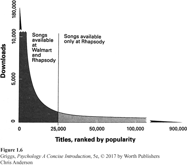
Because unusually high or low scores distort a mean, such distortion occurs for the means of skewed distributions. The mean for a right-skewed distribution is distorted toward the tail created by the few high scores and therefore is greater than the median. The mean for the left-skewed distribution is distorted toward the tail created by the few low scores and therefore is less than the median. When you have a skewed distribution, you should use the median because atypical scores in the distribution do not distort the median. Consider this example from Wheelan (2013). The median annual income for 10 guys sitting at a bar is $35,000 (each earns $35,000 a year). When multibillionaire Bill Gates walks in and sits at the bar, the median remains $35,000. If another multibillionaire comes in and sits at the bar, the median still does not change. Why? Atypical scores do not distort the median. This means that you need to know the type of frequency distribution before deciding which measure of central tendency—mean or median—is more appropriate. Beware, sometimes the inappropriate measure of central tendency for skewed distributions (the mean) is used to mislead you (Huff, 1954).

35

Skewed distributions are also important to understand because various aspects of everyday life, such as medical trends (mortality rates for various diseases), are often skewed. Let’s consider a famous example of the importance of understanding skewed distributions (Gould, 1985). Stephen Jay Gould, a noted Harvard scientist, died of cancer in 2002. However, this was 20 years after he was diagnosed with abdominal mesothelioma cancer and told that this type of cancer had “a median mortality rate of 8 months after diagnosis.” Most people would think that they would only have about 8 months to live if given this median statistic. However, Gould realized that his expected chances depended upon the type of frequency distribution for the deaths from this disease. Because the statistic is reported as a median rather than a mean, the distribution is skewed. Now, if you were Gould, which type of skewed distribution would you want—right or left? Many people at first think they would want left-skewed, but you wouldn’t want this distribution because everyone would be dead within less than a year. Look at its shape in Figure 1.5(b). If it is 8 months from the origin to the median, then it is less than 4 months from the median to the end of the distribution. You would want a severely right-skewed distribution with a long tail to the right, going on for years. This is what Gould found the distribution to be when he examined the medical literature on the disease. The distribution had a tail that stretched out to the right for many years beyond the median, and Gould was fortunate to be out in this long tail, living for 20 more years after getting the diagnosis. When he did die, it was from a different type of cancer (Blastland & Dilnot, 2009).

Gould wrote a famous article called “The Median Isn’t the Message,” in which he argued that his knowledge of statistics saved him from the erroneous conclusion that he would necessarily be dead in 8 months. In confronting his illness, Gould was thinking like a scientist. Such thinking provided him and the many readers of his article with a better understanding of a very difficult medical situation. Thinking like a scientist allows all of us to gain a better understanding of ourselves, others, and the world we all inhabit. Such thinking, along with the accompanying research, has enabled psychological scientists to gain a much better understanding of human behavior and mental processing. We describe the basic findings of this research in the remainder of the book. You will benefit not only from learning about these findings but also from thinking more like a scientist in your daily life.