Chapter 1. Sample 1

1.1 Atomic Orbitals

Organic chemistry is the chemistry of carbon-containing molecules. It is vast in scope, covering all of biology, most of polymer/plastics chemistry, and some of biogeochemistry. Carbon, despite being a relatively rare element in the earth's crust (< 0.03% by weight; > 99% of that is in rocks as carbonate CO₃^2-), offers such value and versatility as a bond-forming element that it has been recruited by evolutionary processes to be THE central element of life. This "carbon-centricity" then makes organic chemistry THE central discipline of chemistry!

At its heart, organic chemistry is the study of carbon-containing compounds' structure, and the relationship between that structure and the compound's chemical properties, like reactivity and stability. In this course, we will spend a good deal of time examining chemical structure, and then we will use that knowledge to help us understand reactivity and stability properties of organic species.

The concept of molecular structure is a vast topic, because molecules are so small that some of the concepts of "structure" that we apply to macroscopic objects just don't apply, or apply differently. In fact, there are several levels of theory that can be used to describe a given molecular structure, each one invented when deficiencies in existing theories became apparent. This "layering" of information makes it somewhat difficult to learn the "rules" of understanding structure, because you can readily run into the problem of not knowing which rules to apply, or which level of theory to use.

In order to simply and eventually unify this topic for our course, we will follow this scheme:

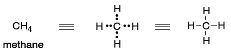
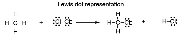
1. Simplest representation: Lewis dot structures (octet rule)
2. Valence bond theory: geometrically correct localized bonds, hybridization, and resonance (ball and-stick molecules)
3. Molecular orbital theory: delocalized molecular orbitals (bonds and antibonds)
4. Localized molecular orbital theory: localized molecular orbitals (localized bonds and antibonds

1.2 Lewis Structures

Gilbert Newton Lewis

What we will find is that we tend to think in (and use) the simplest level of theory adequate to represent the structure in question, while at the same time appreciating that there are higher levels of theory that underpin our simple explanations. So, the familiar Lewis (or line = bond) picture will be adequate for sketching the structures of molecules so we can talk about them and illustrate a chemical reaction.

This type of picture conveys no energy information, and it is somewhat arbitrary in the geometry that we show:

1.3 Valence Bond Theory

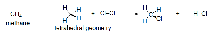
A better representation might evolve as real chemical structures are characterized by spectroscopic techniques (X-ray crystallography is the gold standard for crystalline compounds). These real structures required a re-thinking of the Lewis dot approach so that accurate geometric information can be conveyed. In the case of methane, the geometry actually is determined experimentally to be tetrahedral, not planar. To accommodate this fact, a new theory of bonding was invented, Valence Bond theory.

The starting point for any discussion of bonding models has to be atoms and what they bring to the process of bond formation. The modern description of an atom is as a rough sphere of negatively charged electron density provided by electrons surrounding a tiny core made up of protons (positively charged to balance the negative electron charge) and neutrons – the nucleus. The size/scale difference that the electron cloud and the nucleus impart to an atom can be seen with the simplest atom, hydrogen, H•:

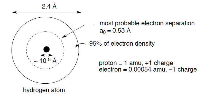
The negatively charged electron and the positively charged proton attract each other with an energy described by Coulomb's law: E = Q1Q2/4πεr, where Q1 and Q2 are the charges, ε = a constant, and r is the distance between the charges. In addition, this electrostatic attraction between electrons and protons accounts for the fundamental reason why atoms join together to form bonds; the positively charged nucleus of one atom is attracted to the negatively charged electrons of a second atom, and vice versa.

1.4 Molecular Orbital Theory

The nucleus is in the middle of the atom, but where is the electron?

HighSlide Content--Click on Image Below

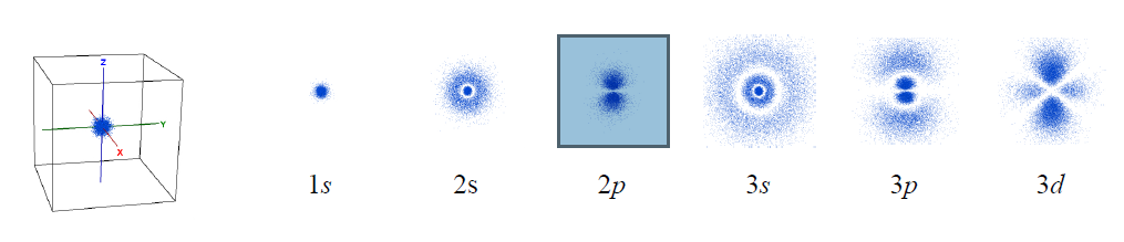
Imagine that we could take thousands of pictures of the electron in the hydrogen atom. Each position of an electron is shown as a blue dot, as illustrated below. The collection of such pictures would describe the probability of finding the electron in various regions of space around the nucleus.

That distribution would vary with the energy of the atom. An electron with relatively high energy will be found in a larger “cloud” (larger average separation from the nucleus) and have some “forbidden” zones (nodes) where the probability of finding it will be zero. You probably have recognized in these pictures the atomic orbitals of hydrogen (1s, 2s, 2p, 3s, 3p, 3d) that you have studied in your general chemistry course.

In reality, we cannot take pictures of electrons, but we can rely on quantum mechanics, one of the monumental intellectual advances in science over the past century, to obtain mathematical functions describing the electron distribution. These functions, called wavefunctions (ψ) as they behave like standing waves, are obtained by solving the Schrödinger equation. The wavefunctions of spherical symmetry (1s, 2s, and 3s) are illustrated below as they “spread” from the nucleus in the center of each plot.

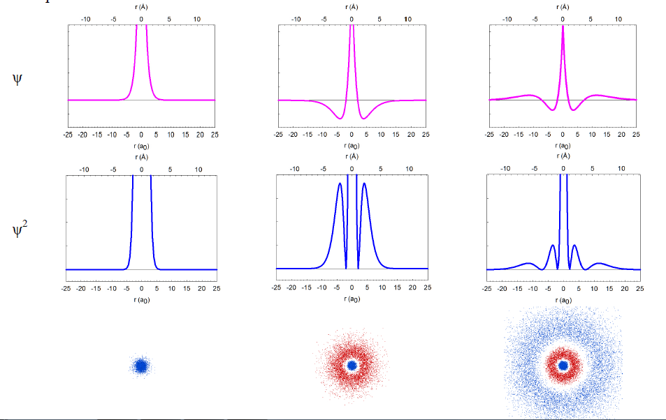
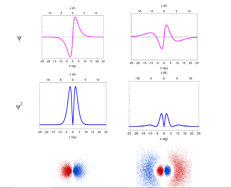
In reality, the wavefunctions themselves have no physical meaning; however, their squares (ψ2) represent electron density, i.e. the probability of finding the electron in a miniscule volume around a given point of space. The relationship of the wavefunctions and electron density plots to our dot displays can be emphasized by showing the dots in red and blue colors to represent the opposite signs of the wavefunction in different regions of space. Similar wavefunctions are obtained for the p orbitals, although they are no longer spherical. For example, the 2pz and 3pz orbitals lie along the zaxis.

We can make several general observations about these atomic orbitals. First of all, they are really 4-dimensional constructs: for every point in space ([x,y,z]) a value of the wavefunction (or its square) is specified. Thus, three of an orbital's dimensions are the standard geometric coordinates. Although the functions stretch to infinity, the total probability of finding an electron in an orbital is unity, as the electron has to be somewhere around the nucleus. We call such functions normalized. The wavefunctions can have positive and negative values in different regions in space, and have zero values in regions around the nucleus where electrons are not allowed (nodes). Note that the electron density is always positive (i.e., the square of the wavefunction) or zero. All orbitals encompass the same space around the nucleus, yet they are quite distinct. They have zero overlap with each other. We call them orthogonal.

The overlap of wavefunctions (or orbitals) has a special meaning in quantum chemistry, extending beyond the measure of simple spatial interpenetration. Just for the purposes of our graphical simplification, we can think of the overlap as a common space occupied by two orbitals, but explicitly taking into account the algebraic sign of that "space". Consider the 2s and 2p orbitals of hydrogen, for example. The "common space" (i.e., the p orbital lobe that overlaps with the s orbital) on the left (+/+ or -/-) has the opposite sign than the "common space" on the right (+/-). The two contributions cancel, and there is no net overlap be tween these orbitals.

1.5 Localized Molecular Orbital Theory

There is another “dimension” to the orbitals that must be explicitly taken into account: orbital energy. An electron has the same total energy anywhere within the orbital, but different orbitals may have different energies. For example, the 1s and 2s orbitals have different energies, even though they occupy approximately the same region of space around the nucleus. All three 2p orbitals have the same energy (they are degenerate) even if they are aligned along di fferent axes (2px, 2py, 2pz).

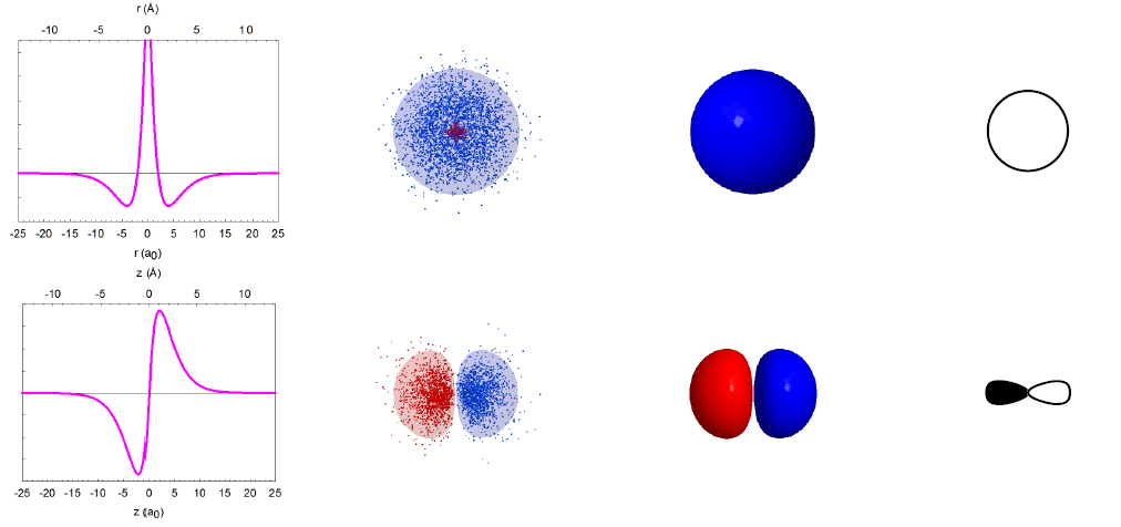
For convenience of presentation, we will replace the mathematical functions with simplified graphical representations in our qualitative consideration of orbitals and orbital interactions. First of all, we will concentrate only on 90% of the electron density in a given orbital. We will draw a boundary surface enclosing such a fraction of the electron density and mark it (by color or shading) with the algebraic sign of the underlying wavefunction. We will neglect all variations of the electron density, including any nodes, within the orbital.

We will further simply our analyses by limiting our menagerie of orbitals to just those ones that play decisive roles in the structure and chemistry of organic molecules; 1s for hydrogen, 2s, and three 2p orbitals for all elements of the second row of the periodic table.

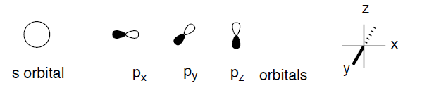
We note that d orbitals just don't come into use for organic species very often. All orbitals of one particular type will have the same overall shape, but they will differ in size (and energy). The orbitals of elements with higher effective nuclear charge (i.e., more electronegative elements, to the right in the periodic table) will be smaller and will have lower energy. The orbital size will grow with the increase in the principal quantum number (i.e., 1s < 2s < 3s). Atoms lower in the periodic table will have bigger orbitals. The Pauli exclusion principle limits the number of electrons in any orbital to a maximum of two with opposite spins. Thus, any orbital can be occupied by 0, 1, or 2 electrons.