Concept 41.2: Solar Energy Input and Topography Shape Earth’s Physical Environments

Earth’s physical environments vary enormously—from hot to cold, wet to dry, aquatic to terrestrial, salt water to fresh water. To this variation across space we must add variation over time, on scales from the very slow coming and going of oceans, mountains, or ice ages to the very fast shifts in temperature as clouds pass overhead. On the short time scales that we humans experience, physical conditions depend largely on solar energy input, which drives the circulation of the atmosphere and the oceans. Patterns of input and circulation determine whether a particular place at a particular time of year tends to be hot or cold, wet or dry—and as a consequence, the types of organisms found in that place.

Variation in solar energy input drives patterns of weather and climate

All of us are familiar with weather, the atmospheric conditions—temperature, humidity, precipitation (rainfall or snowfall), and wind direction and speed—that we experience at a particular place and time. Averaged over long periods, the state of these atmospheric conditions and their pattern of variation over time constitute the climate of a place. In other words, climate is what you expect; weather is what you get. We and other organisms respond to both weather and climate. Responses to weather are usually short-term: animals may seek shelter from a sudden rainstorm (human animals open their umbrellas), and plants may close their stomata (small openings in the leaf epidermis) on a hot summer day to reduce water loss from their tissues. Responses to climate, by contrast, tend to involve adaptations that prepare organisms for expected conditions. Organisms in hot climates can tolerate heat; those that inhabit seasonal climates use cues such as day length to prepare for an impending hot, cold, or dry season.

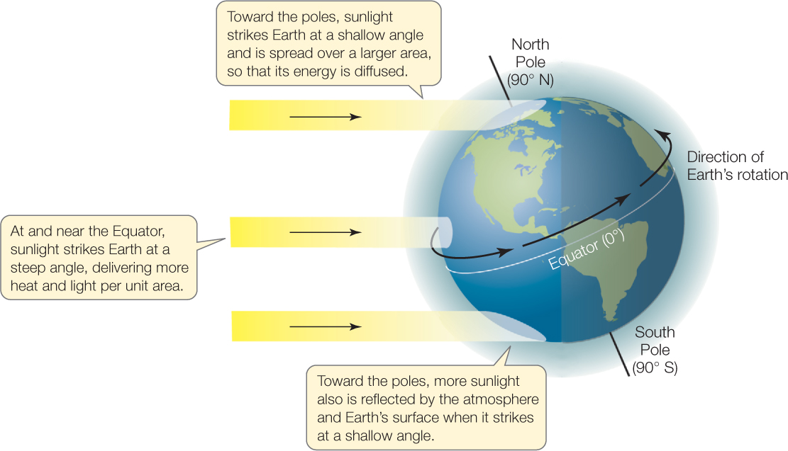
Some global patterns of climate stem from variation in solar energy input over space. Because Earth is spherical, the sun’s rays strike the planet at a shallower angle near the poles than near the equator (FIGURE 41.3). This difference results in less solar energy input at high latitudes (near the poles) than at low latitudes (near the equator), for two reasons. First, the energy of rays of sunlight is spread over a larger surface area at high latitudes. Second, more sunlight is reflected back into space by the atmosphere and Earth’s surface when sunlight strikes at a shallow angle. A consequence is that air temperatures decrease from low latitudes to high latitudes. Averaged over the course of a year, air temperature drops by about 0.8°C with every degree of latitude (about 110 km) north or south of the equator.

Figure 41.3: Solar Energy Input Varies with Latitude The angle of incoming sunlight affects the amount of solar energy that reaches a given area of Earth’s surface. On average, sunlight strikes Earth’s surface at a steeper angle at low than at high latitudes. This results in greater input of energy at low (i.e., equatorial) latitudes because the energy is spread over a smaller area and because less sunlight is reflected back into space by the atmosphere and land surface.

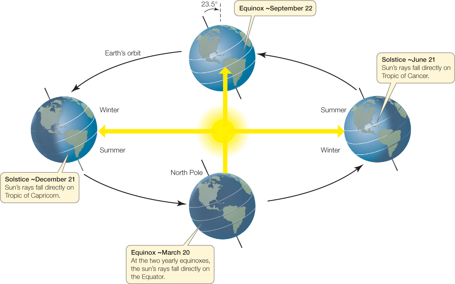
At any given place, the sun’s input also varies through the year, causing seasonal variation in climate. This seasonality is a consequence of the 23.5° tilt of Earth’s axis of rotation relative to the plane of its yearly orbit around the sun. The tilt causes different latitudes to receive their greatest solar energy input at different times of the year (FIGURE 41.4). At the solstice in late June, the North Pole tilts toward the sun, and the sun is directly above the Tropic of Cancer (latitude 23.5° N): the Northern Hemisphere experiences summer, with its long days and warm temperatures. At the solstice in late December, the North Pole points away from the sun, the sun is directly above the Tropic of Capricorn (latitude 23.5° S), and the climate pattern is reversed: it is summer in the Southern Hemisphere and winter in the Northern Hemisphere. At the equinoxes in late March and late September, the sun is directly above the equator, and both hemispheres experience equal lengths of day and night. These seasonal variations in solar input are relatively small at the equator and become more pronounced toward the poles.

Figure 41.4: The Tilt of Earth’s Axis of Rotation Causes the Seasons As Earth orbits the sun, the North Pole alternately tilts toward and away from the sun. This tilt causes the latitude of greatest solar energy input to shift between the Tropics of Cancer (23.5° N) and Capricorn (23.5° S) over the course of a year.

The circulation of Earth’s atmosphere redistributes heat energy

The yearly input of solar energy is greatest in the tropics (the latitudes between the Tropics of Cancer and Capricorn) and decreases poleward. This latitudinal gradient in solar input drives the vast circulation patterns of Earth’s gaseous atmosphere.

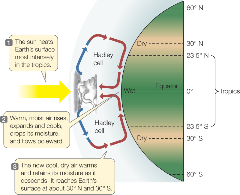
As the sun beats down on the tropics, the air there heats up—its molecules move faster (temperature is a measure of disordered molecular motion), colliding and pushing one another farther apart (see Concept 2.5). The heated air expands, becoming less dense and more buoyant, and rises. As it rises, it continues to expand and cool adiabatically (this is the principle on which an air conditioner works: when compressed gas is allowed to expand, it cools). The air rises to a level at which the surrounding air has its same temperature and density. Because tropical air gets so warm, it ascends to great altitudes before it stops rising.

Rising tropical air creates a vacuum that pulls in cooler, denser surface air from the north and south. As that air in turn heats, expands, and rises, it pushes the cool air above it to the side. As this air aloft moves away from the tropics, it radiates heat to outer space, becoming more dense and less buoyant. It sinks back toward Earth, is compressed by the overlying atmosphere, and warms adiabatically (the reverse of adiabatic cooling). It reaches Earth’s surface at latitudes of roughly 30° N and 30° S, at which point some of it flows back toward the equator to replace air that is rising in the tropics. Thus it forms two cycles of vertical atmospheric circulation—one north and one south of the equator—called Hadley cells (FIGURE 41.5).

Figure 41.5: Tropical Solar Energy Input Sets the Atmosphere in Motion Intense sunlight in the tropics drives a vertical pattern of atmospheric circulation that reaches the subtropics and that results in high precipitation near the equator.

The Hadley cell circulation produces strong latitudinal patterns of precipitation. As water molecules in the tropics (most notably the oceans) absorb the intense sunlight there, they evaporate, so the air that rises in the tropics is rich in water vapor. As this warm, moist air expands and cools, fewer water molecules are moving fast enough to bounce apart after they collide. Instead, they form droplets of liquid water (or ice crystals), which grow and—when massive enough—fall to the ground as precipitation. Thus the warm, rising air of the Hadley cells drops most of its moisture near the equator as rain. The high-altitude air that eventually descends near 30° N and 30° S is largely depleted of water; moreover, because it warms as it descends and is compressed, the little water that remains stays in a gaseous state. Earth’s great deserts are located around these latitudes.

Not all the descending air in the Hadley cells returns immediately to the tropics. Some of it continues to flow toward the poles, encountering and overriding frigid, dense polar air that is flowing equatorward as part of polar circulation cells that are smaller and weaker than the Hadley cells. The interaction of these warm and cold air masses generates the spinning winter storms that sweep from west to east through the middle latitudes between the tropics and the polar regions.

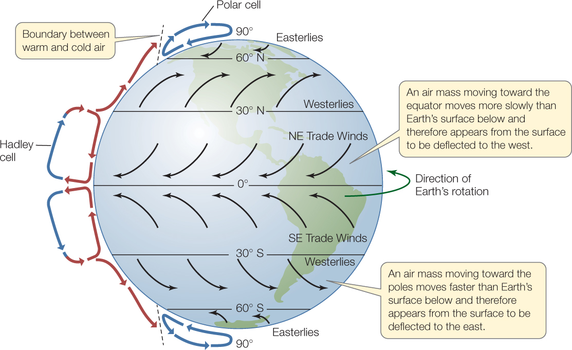
To better understand these storms and other patterns of horizontal air movement, we must consider one more thing—Earth’s rotation on its axis from west to east (see Figure 41.3). We have already seen that the latitudinal gradient in solar input creates a latitudinal, or north–south, movement of air. The planet’s rotation adds an east–west component to air movement. Because Earth is a sphere, the rotation of its surface is fastest at the equator, where its circumference is greatest, and slower toward the poles. Surface air that is not moving north or south is carried eastward at the same speed as the surface beneath it. But air that is moving toward the equator lags behind the faster-moving surface, and therefore appears from the surface to be deflected to the west. Conversely, air that is moving poleward races ahead of the surface and appears to be deflected to the east. This Coriolis effect causes prevailing surface winds to blow from east to west in the tropics (the northeast or southeast trade winds, so called because of their importance during the era of trade by sailing ships), from west to east in the middle latitudes (the westerlies), and from east to west again above 60° N and 60° S latitude (the easterlies; FIGURE 41.6). The Coriolis effect also leads to the rotation of air characteristic of middle-latitude storms.

Figure 41.6: Global Atmospheric Circulation and Prevailing Winds Because the speed of rotation of Earth’s surface decreases with latitude, air flowing toward the equator lags behind the surface beneath it, whereas air flowing toward the poles moves faster than the surface beneath it. The resulting Coriolis effect explains patterns of prevailing surface winds.

These aspects of atmospheric circulation combine to affect climate patterns by transferring an immense amount of heat energy from the hot tropics to the cold poles. Without this transfer, the poles would sink toward absolute zero in winter, and the equator would reach fantastically high temperatures throughout the year.

Ocean circulation also influences climate

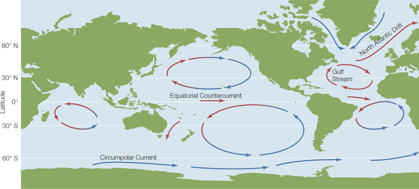
The prevailing surface winds and Coriolis effect drive massive circulation patterns in the waters of the oceans, called currents, which carry materials, organisms, and heat with them. In the northern tropics, the trade winds drag surface water toward the west. When this water nears the western edge of an ocean basin, much of it flows northward, only to be turned to the east by the Coriolis effect and, at higher latitudes, by drag from the westerlies of the northern middle latitudes. This eastward flow turns south along the western edge of the continents and then westward again, completing a clockwise circuit, or gyre. The pattern in the Southern Hemisphere is essentially a mirror image of that just described, with surface circulation moving in counterclockwise rather than clockwise rotation (see Figure 41.7). The westward-flowing tropical water that is not caught up in these gyres flows back to the east in an equatorial countercurrent.

As they move poleward, tropical surface waters transfer heat from low to high latitudes, adding to the heat transfer that accompanies atmospheric circulation. The Gulf Stream and North Atlantic Drift, for example, bring warm water from the tropical Atlantic Ocean and the Gulf of Mexico north and east across the Atlantic (FIGURE 41.7), which warms the air above the North Atlantic. Westerlies then carry this air across northern Europe, moderating temperatures there. The effect on organisms is dramatic: polar bears roam the shores of Hudson Bay in Canada but are missing from comparable latitudes in Scotland or Sweden.

Figure 41.7: Ocean Surface Currents Ocean surface currents are characterized by giant patterns (gyres) of clockwise rotation in the Northern Hemisphere and counterclockwise rotation in the Southern Hemisphere, caused by frictional drag from prevailing winds (see Figure 41.6), the Coriolis effect, and deflection at the edges of continents.

Surface currents are not the entire story, however. Gradients in water density caused by variation in temperature and salinity cause surface waters to sink in certain regions, forming deep currents. These deep currents return to the surface in areas of upwelling, completing a vertical ocean circulation. Thus oceanic circulation, like atmospheric circulation, is three-dimensional.

Oceans and large lakes moderate Earth’s terrestrial climates because water has a high heat capacity, as we saw in Concept 2.2. This means that the temperature of water changes relatively slowly as it exchanges heat with the air it contacts and as it absorbs or emits radiant energy. As a result, water temperatures fluctuate less with the seasons and with the day–night cycle than do land temperatures, and the air over land close to oceans or lakes also shows less seasonal and daily temperature fluctuation.

Topography produces additional environmental heterogeneity

Earth’s surface is not flat; it is crumpled into mountains, valleys, and ocean basins. This variation in the elevation of Earth’s surface, known as topography, affects the physical environment.

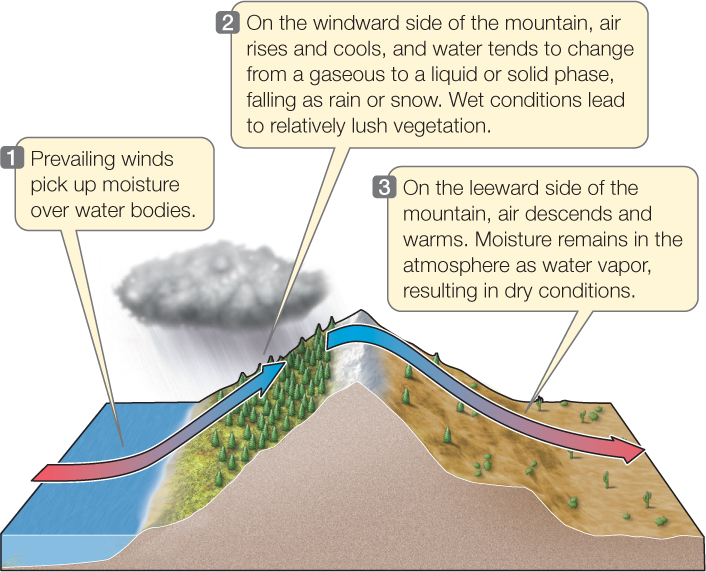
Mountains, for example, are “weather formers.” Because rising air expands and cools adiabatically, temperatures become cooler as elevation (distance above sea level) increases. If you climb a mountain, you will find that the temperature drops by about 1°C for each 220 meters of elevation gained. Where prevailing winds encounter a mountain range, air flows up the windward side of the range (the side facing into the wind). As the air cools, water vapor may condense or crystallize and fall as rain or snow. The leeward side of the mountain range (the side away from the wind) receives little precipitation because air descending on that side warms and retains any remaining water in a gaseous state. Thus the mountain range is said to form a rain shadow (FIGURE 41.8). The difference in precipitation fosters more luxuriant growth of plants on the windward side than on the leeward side.

Figure 41.8: A Rain Shadow Precipitation tends to be lower on the leeward side of a mountain range than on the windward side.

APPLY THE CONCEPT: Solar energy input and topography shape Earth’s physical environments

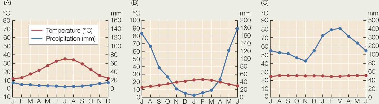
Shown below are climate diagrams for three different localities. (Note the discontinuity in the precipitation axis in graph C.) Using the information in these diagrams and what you’ve learned about factors that determine climate, answer the following questions and explain the logic that led to your answer.

1. Which locality is near the equator?
2. Which locality has the greatest seasonality in temperature?
3. Which locality has the longest growing season?
4. Which locality is in the Northern Hemisphere?

Topography also influences physical conditions in aquatic environments. The velocity of water flow, for example, is dictated by topography: water flows rapidly down steep slopes, more slowly down gradual slopes, and pools as lakes, ponds, or oceans in depressions. The depth of a water-filled depression determines the gradients of many abiotic factors, including temperature, pressure, light penetration, and water movement (see Figure 41.13).

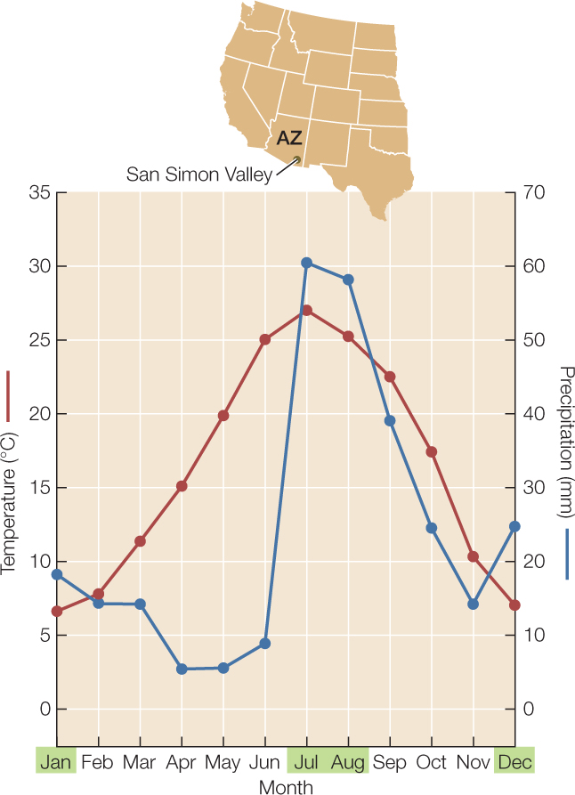
Climate diagrams summarize climates in an ecologically relevant way

The climate at any location can be summarized in a climate diagram. Recognizing that ecological processes are strongly influenced by temperature and moisture, the German biogeographer Heinrich Walter superimposed graphs of average monthly temperature and average monthly precipitation through the year. He scaled the axes of the two graphs to incorporate the rule of thumb that plant growth requires at least 20 millimeters of precipitation per 10°C of temperature above freezing (0°C). This scaling makes it easy to see when conditions allow terrestrial plant growth—when temperature is greater than 0°C and the precipitation line is above the temperature line. This period is known as the growing season (FIGURE 41.9).

Figure 41.9: Climate Diagrams Summarize Climate in an Ecologically Relevant Way Climate diagrams traditionally combine graphs of average temperature (left axis) and average precipitation (right axis) throughout the year, as shown here for San Simon Valley near the Arizona–New Mexico border. The summer solstice at the location in question (late June in the Northern Hemisphere, late December in the Southern hemisphere) is placed at the center of the diagram. The axes are scaled such that precipitation favors plant growth when the precipitation line is above the temperature line. The months highlighted in green are typically favorable for plant growth.

The patterns in the physical world that we have just discussed limit where organisms can live. For this reason, they strongly influence biogeography—the spatial distributions of species.