Concept 42.4: Populations Grow Multiplicatively, but the Multiplier Can Change

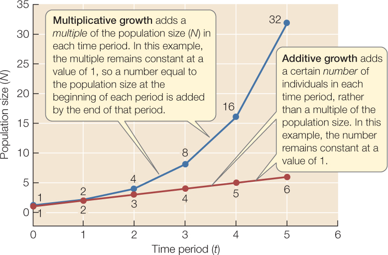
We saw in Concept 42.2 that a population will grow as long as the per capita growth rate, r, is greater than zero. Recall also that r refers to a specific period of time (it might be a day, a week, or a year, depending on the species) over which we have estimated per capita birth and death rates. During this period the population will add a number of individuals that is precisely r times its initial size. In other words, growth is multiplicative. We saw this in Equation 42.3, which states that N_t+1 = N_t + rN_t. What may not be obvious at first is that this pattern continues in the next time period: the population will again add a multiple r of its numbers, since N_t+2 = N_t+1 + rN_t+1. Because N_t+1 was already larger than the initial population N_t, this means that an ever-larger number of individuals is added in each successive period, as long as the multiplier r remains constant.

Multiplicative growth with a constant r differs dramatically in its form from additive growth, in which a certain number (rather than a certain multiple) is added in each period:

Multiplicative growth with constant r can generate large numbers very quickly

We naturally tend to think in terms of additive growth, so multiplicative growth with an unchanging, positive multiplier astonishes us with the phenomenal numbers it can generate in a short time. For example, in 1911 L. O. Howard, then chief entomologist (insect scientist) of the U.S. Department of Agriculture, estimated that a pair of flies reproducing for the first time on April 15 would give rise to a population of 5,598,720,000,000 adults by September 10 if all the offspring survived and reproduced. Other entomologists disagreed with Howard’s calculation—they pegged the number much higher!

Charles Darwin was well aware of the power of multiplicative growth:

This ecological struggle for existence, fueled by multiplicative growth, is an essential part of natural selection and adaptation.

Populations growing multiplicatively with constant r have a constant doubling time

Multiplicative growth characterizes many phenomena that affect our everyday lives, such as interest-bearing bank accounts, fossil-fuel consumption, and radioactive decay (see Figure 18.1). Our tendency to think in additive terms impedes our ability to comprehend these phenomena and to understand their practical implications. For example, how much more money will we have in 5 years if we invest $1,000 in a bank account that earns 2 percent per year as opposed to 1 percent per year? How does the drop in the per capita growth rate from 2.20 percent per year in 1963 to the current 1.14 percent change our estimates of the future size of the global human population? Answering such questions requires an understanding of multiplicative growth.

Multiplicative growth with a constant r has a very striking property: a constant doubling time. A population growing in this way adds an ever-increasing number of individuals as time goes on. At some specific time, the number added exactly equals the initial population, and the population has doubled. As long as r does not change, the time the population takes to double will also remain constant. The doubling time depends on r—it gets shorter as r increases.

It is easy to see the implications of multiplicative growth with a constant, positive r if we think in terms of doubling times. For example, by doing so a municipality would see that even a seemingly small but constant growth rate of 3 percent per year would mean that its population would double every 23 years—and that its sewage treatment capacity and other such municipal services would need to do the same.

Density dependence prevents populations from growing indefinitely

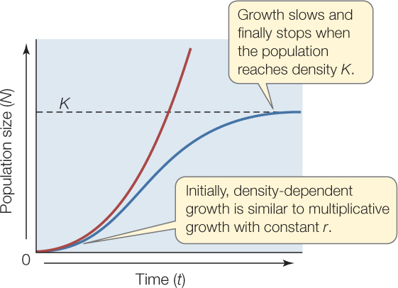
If populations grow multiplicatively, why isn’t Earth covered with flies, or any other organism? It turns out that populations do not grow multiplicatively with constant r for very long. Instead of continuing to increase (as in the red J-shaped curve in the graph below), population growth eventually slows, and population size usually reaches a more or less steady size (as in the blue S-shaped curve):

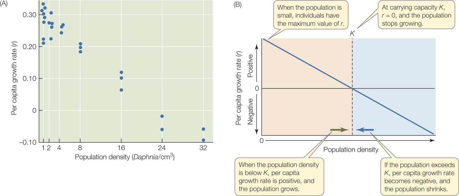
Why do populations stop growing? Upon examination, we see that even though the population still adds a multiple of its previous size in each time period, the multiplier r, which determines what is added to the population, changes, rather than remaining constant. As the population becomes more crowded, r decreases—in other words, r is density dependent (FIGURE 42.8A). At low population densities, per capita growth rates are at their highest. As the population grows and becomes more crowded, per capita birth rate tends to decrease and death rate to increase, and so r decreases toward zero. When r = 0, the population stops changing in size—in other words, it reaches an equilibrium size. That size is called the carrying capacity, or K (FIGURE 42.8B). K can be thought of as the number of individuals that a given environment can support indefinitely. If individuals are added to the population so that it exceeds the carrying capacity, the per capita growth rate becomes negative, and the population shrinks. If the population falls below K, the per capita growth rate becomes positive, and the population grows (see Figure 42.8B).

Figure 42.8: Per Capita Growth Rate Decreases with Population Density (A) The decline in r as population density increases, as measured in a population of a small crustacean, Daphnia pulex (see Figure 42.10). (B) Schematic representation of density-dependent growth, in which r declines linearly with population density. This graph is an idealization—few species follow it exactly. For example, close inspection of (A) suggests that the decline in r for Daphnia pulex is not precisely linear.

APPLY THE CONCEPT: Populations growing multiplicatively with constant {em}r{/em} have a constant doubling time

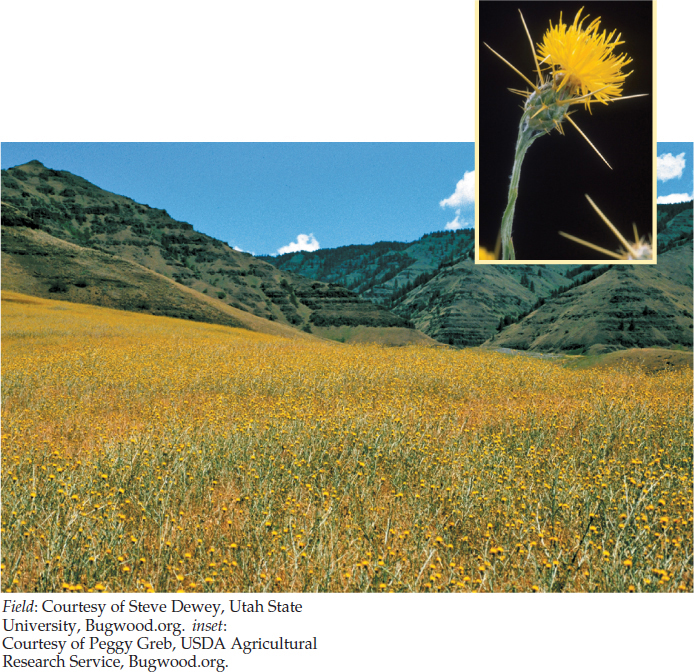
Yellow star-thistle (Centaurea solstitialis) is a spiny annual plant native to the Mediterranean region. The species has invaded several regions of the United States. It is a noxious weed that is unpalatable to livestock (including American bison). Jane, the rancher, discovers that 1 hectare of her 128-hectare pasture has been invaded by star-thistle. A year later, she finds that the weed population has grown to cover 2 hectares.

1. Based on the information above, how many hectares do you predict the star-thistle population will cover in 1, 2, and 3 more years if the population is growing additively by a constant number? How many hectares if the population is growing multiplicatively with constant r?
2. Imagine that Jane discovers the star-thistle population only after it has already covered 32 hectares of her pasture. How many years does she have until the weed completely covers the pasture if its population is growing additively by a constant number each year? How many years does she have if it is growing multiplicatively with constant r?

The invasive yellow star-thistle is noxious to grazing livestock.

Why does r decrease with crowding? When used by one organism, a resource becomes unavailable to other organisms. Therefore, as population density increases, each individual gets a smaller piece of the resource “pie” and has less to allocate to its life functions (see Figure 42.5). Per capita birth rate decreases, per capita death rate increases, and therefore r decreases with population density. Once again it is useful to spell this out:

• Per capita growth rate = the maximum possible value in uncrowded conditions − an amount that is a function of density

When population density reaches K, the carrying capacity, the average individual has just the amount of resources it needs in order to produce enough offspring to have exactly replaced itself by the time it dies. When density is less than K, the average individual can more than replace itself; when density is greater than K, the average individual has fewer resources than it needs to replace itself.

Now we are prepared to return to the question posed at the end of Concept 42.1: Why do species abundances vary in time and space?

Changing environmental conditions cause the carrying capacity to change

We have learned that resource availability in the environment affects an individual’s success in acquiring resources (see Figure 42.4), and that physical conditions affect the costs of maintenance (see Figure 42.5). If these factors vary over space, then the carrying capacity will vary over space as well.

Similarly, if resource availability or environmental conditions are good in one year but bad in another, the population will find itself alternately above and below the current carrying capacity. As a result, populations will fluctuate around an average K over time. Figure 42.2 illustrates this dynamic for rodents and ticks in Millbrook, New York. Rodent densities tend to increase following years of high acorn production because the rodents have enough food to produce many offspring, and they tend to decrease following poor acorn years. Similarly, nymphal tick densities go up and down following high and low rodent years, respectively, because host abundance determines the success of larval ticks in obtaining a blood meal. These increases and decreases are not immediate—there is a delay while acorns are converted into newborn rodents, and while newly fed larval ticks molt into nymphs.

A look back at Table 42.1 shows how temporal changes in the environment affected the fecundity of a group of 210 common cactus finches born on Isla Daphne in 1978. Notice that females produced no surviving young when they were 7 and 8 years old. These years followed a severe drought in 1985 that limited production of the seeds the finches eat. Conversely, fecundity was unusually high when the finches were 5 and 9 years old. These were the unusually wet years of 1983 and 1987, when food was plentiful.

Technology has increased Earth’s carrying capacity for humans

The human population is unique among populations of large animals. Not only has it continued to grow, it has grown at an ever-faster per capita rate until very recently, as is indicated by its steadily decreasing doubling times (FIGURE 42.9A). The current population multiplier, or per capita growth rate (r), is somewhat above 1.1 percent per year, lower than the peak of 2.2 percent reached in 1963, because birth rates have declined faster than have death rates over the past 50 years. Even if this recent trend in r continues, however, the human population is projected to grow to 8 billion by 2025.

Figure 42.9: Human Population Growth Advances in technology have allowed the human population to grow at an ever-faster per capita rate.

The human population growth rate has jumped with every technological advance that has raised carrying capacity by increasing food production (thereby increasing per capita birth rate, b) or by improving health (thereby reducing per capita death rate, d). The first jump occurred with the rise of agriculture (about 10,000 years ago). In the nineteenth and twentieth centuries, advances in sanitation and the development of vaccines and antibiotics decreased death rates to an unprecedented low level (FIGURE 42.9B). Finally, the “Green Revolution” in agriculture more than doubled world grain production between 1950 and 1984. These increases in r correspond to shorter and shorter doubling times (see the table in Figure 42.9A) until very recently.

Human ingenuity has repeatedly stymied attempts to predict the future of the human population. The most famous attempt was that of Thomas Malthus, whose Essay on the Principle of Population, first published in 1798, provided Charles Darwin with a critical insight for his theory of natural selection. Malthus reasoned that the human population was growing multiplicatively, whereas its food supply was growing additively. He predicted that food shortages would limit human population growth, which he estimated would peak by the end of the nineteenth century. Malthus could not, of course, have anticipated the effects of medical discoveries and the Green Revolution.

Many believe that the human population has now overshot its long-term carrying capacity. They give two reasons. First, most twentieth-century technological advances relied on abundant fossil fuels instead of renewable biomass and muscle power, and fossil fuels are not renewable. Maintaining current levels of agricultural production depends heavily on fertilizers derived from natural gas, pesticides derived from oil, and petroleum-fueled engines that pump irrigation water, till the soil, and process and transport food. Similarly, the manufacture and distribution of medicines and diagnostic machinery depends on fossil fuels. World production of crude oil has continued to rise but cannot do so indefinitely because reserves are finite, and the same is true of coal, natural gas, and other fossil fuels. Eventually these fuels will be depleted.

A second reason many believe that our carrying capacity will decrease in the near future is the climate change and degradation of Earth’s ecosystems that have been a consequence of our recent population expansion. We will consider these topics further in Chapters 44 and 45.

Population ecology tells us that the growth trajectory of the global human population will change only when birth and death rates change. If the human population has indeed exceeded its long-term carrying capacity, it will ultimately have to shrink. We can bring this about voluntarily if we continue to reduce our per capita birth rate. The less pleasant alternative is to wait for the Four Horsemen of the Apocalypse—famine, pestilence, war, and death—to achieve a sustainable human population size.

So far we have considered the effects of two universal demographic processes—birth and death—on populations. But the dynamics of many populations are also influenced by the movement of individuals among populations. Such “open” populations grow when immigrants enter from the outside world and shrink when emigrants leave. Immigration and emigration affect populations in important ways.