15.3 GENOMEWIDE STUDIES OF GENETIC VARIATION

Restriction enzymes are extremely useful for some purposes, but their utility as a tool for studying genomewide genetic variation is limited because they reveal only sequence variation in restriction sites or differences in the distances between adjacent restriction sites. In this section, we examine methods by which genetic differences in any individual nucleotide can be studied.

15.3.1 Single-nucleotide polymorphisms (SNPs) are single base changes in the genome.

One of the most common types of genetic variation is a difference in a nucleotide at a specific site. A single-nucleotide polymorphism (SNP) is a site in the genome where there is a base-pair difference among chromosomes that is common enough to be present in a random sample of 50 diploid individuals. The differences among the hemoglobin alleles are SNPs. The A, S, and C alleles differ from each other at just one nucleotide site (see Fig. 15.1).

Figure 15.7: Single-nucleotide polymorphisms (SNPs). A SNP in the region neighboring OCA2 is strongly associated with blue eyes.

Eye color is also associated with a SNP. The blue-eyed phenotype results from reduced expression of a gene called OCA2, which encodes a membrane protein involved in the transport of small molecules including the amino acid tyrosine, which is a precursor of the melanin pigment associated with brown eyes. Although more than a dozen alleles of OCA2 are known that have an amino acid replacement in the protein, none of these results in blue eyes.

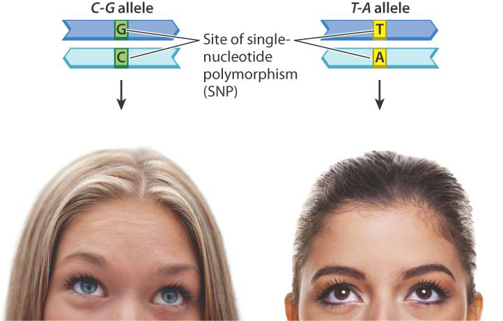
The SNP nucleotide implicated in blue eyes is a C–G base pair in one allele. The other common variant is a T–A, which is not associated with blue eyes (Fig. 15.7). In one study, the homozygous C–G genotype was found in 94% of 183 individuals with blue eyes and in only 2% of 176 individuals with brown eyes. This strong association is quite unexpected because the SNP associated with blue eyes is a noncoding SNP present in an intron of a neighboring gene. The proposed mechanism for the association is that the C–G allele makes the adjacent OCA2 gene less accessible to transcription factors, thereby reducing the amount of the transporter protein and consequently the production of melanin in the iris. The proposed mechanism may be right or wrong; this example emphasizes that scientists have much to learn about the possible phenotypic effects of noncoding DNA.

The C–G versus T–A SNP is typical of most SNPs in that only two of the four possible base pairs are present in the population at any appreciable frequency.

15.3.2 How can genetic risk factors be detected?

SNPs result from point mutations, the most frequent type of mutation. A point mutation is the substitution of one base pair for another in double-stranded DNA (Chapter 14). Each of us is genetically unique partly because of the abundance of SNPs in the human genome. There are approximately 3 million SNPs that distinguish any one human genome from any other. SNPs are abundant in the genomes of most species; some are thought to be the main source of evolutionary innovation, and others are major contributors to inherited disease. Practically speaking, SNPs are important because they can be used to detect the presence of a genetic risk factor for a disease before the onset of the disease. For example, the ability to detect the β-globin SNPs shown in Fig. 15.1 allows prenatal identification of the β-globin genotype of a fetus.

While there is great interest in developing ultrafast DNA sequencing machines that can determine anyone’s personal genome quickly at relatively low cost, between any two genomes 99.9% of the nucleotides are identical. An alternative is to focus on genotyping just SNPs. As many as one million SNPs at different positions in the genome can be genotyped simultaneously, and the genotyping can be carried out on thousands or tens of thousands of individuals. Such massive genotyping allows any SNP associated with a disease to be identified, which is especially important for complex diseases affected by many different genetic risk factors (Chapter 18).

What does it mean to say that a SNP is associated with a disease? It means that individuals carrying one of the SNP alleles are more likely to develop the disease than those carrying the other allele. The increased risk depends on the disease and can differ from one SNP to the next. Sickle-cell anemia affords an example at one extreme of the spectrum of effects. In this case, the T–A base pair in the S allele of the β-globin gene is the SNP that results in the amino acid replacement of glutamic acid with valine in the protein. Because SS individuals always have sickle-cell anemia, it would be fair to say that homozygous S “causes” sickle-cell anemia.

But except for inherited diseases due to single mutant genes, which are usually rare, the vast majority of SNPs implicated in disease increase the risk only moderately, typically by 10% to 50% as compared with individuals lacking the risk factor. We then say that the SNP is “associated” with the disease, since the SNP alone does not cause the disease but only increases the risk. For heart disease, diabetes, and some other diseases, many SNPS at different places in the genome, as well as environmental risk factors, can be associated with the disease. Usually, genetic and environmental risk factors act cumulatively: the more you have, the greater the risk.

As emphasized in the case of Claudia Gilmore’s genome, certain SNPs in the BRCA1 and BRCA2 genes are associated with an increased risk of breast and ovarian cancers. Women who carry a mutation in either of these genes can minimize their risk by frequent mammograms and other tests. Both genes are large—BRCA1 codes for a protein of 1863 amino acids and BRCA2 for one of 3418 amino acids—and many different mutations in these genes can predispose to breast or ovarian cancer. In certain high-risk populations, however, such as Ashkenazi Jews, only a few mutations predominate, and the SNPs associated with these mutations can be detected easily and efficiently.

15.3.3 SNPs can be detected by DNA microarrays.

A widely used method for SNP genotyping is shown in Fig. 15.8. The technique involves a DNA microarray, which consists of a waferlike supporting surface about the size of a postage stamp to which are attached millions of different oligonucleotides, short, single-stranded DNA molecules of known sequence. Microarrays have many applications in biology, one of which is the detection of SNPs. For each SNP, researchers design oligonucleotides that contain a base in the middle that is complementary to one or the other of the SNP alleles. In the example shown in Fig. 15.8a, the bases on the oligonucleotide are G and C, which complement one SNP allele, and A and T, which complement the other. The flanking bases are complementary to those in both SNP alleles, which are the same. Although for clarity each oligonucleotide is shown as a single strand in Fig. 15.8a, there are actually millions of identical copies of each oligonucleotide deposited at each spot on the microarray.

Figure 15.8: SNP genotyping. SNPs can be genotyped by observing their pattern of hybridization with oligonucleotides on a microarray.

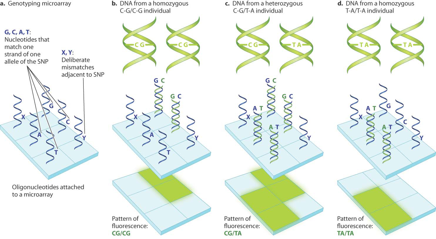
Once a microarray with oligonucleotides complementary to both SNP alleles has been constructed, researchers add single-stranded DNA taken from an individual. Recall that DNA hybridization involves two single-stranded DNA molecules forming a double-stranded DNA molecule (Chapter 12). Under suitable conditions of hybridization, DNA fragments from individuals homozygous for the C–G allele will hybridize only with the oligonucleotides that contain G or C (Fig. 15.8b) and those from individuals homozygous for the T–A allele will hybridize with the oligonucleotides that contain A or T (Fig. 15.8d). The DNA fragments from heterozygous C–G/T–A individuals will hybridize with all the complementary oligonucleotides (Fig. 15.8c). The DNA fragments are usually labeled with a fluorescent dye, and any fragment that hybridizes with an oligonucleotide will fluoresce at that site.

The patterns of fluorescence are shown beneath the microarrays in Fig. 15.8. The key point is that each SNP genotype yields a unique pattern of fluorescence. DNA microarrays also include oligonucleotides that serve as experimental controls (important in any experiment) to ensure that the correct SNP has been identified. These contain deliberate mismatches adjacent to the site of the SNP. The control oligonucleotides in Fig. 15.8 are denoted X and Y; and they are expected not to show any fluorescence.

15.3.4 Copy-number variation constitutes a significant proportion of genetic variation.

Figure 15.9: Copy-number variation in a region of a chromosome.

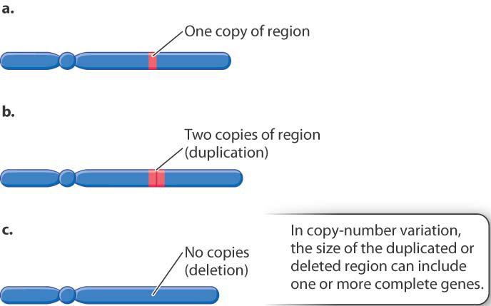
Genotyping microarrays are useful for detecting copy-number variation (CNV), the differences among individuals in the number of copies of a region of the genome. In contrast to the short repeats characteristic of VNTRs, the regions involved in CNVs are large and may include one or more complete genes. An example is shown in Fig. 15.9. In this case, a region of the genome that is normally present in only one copy per chromosome (Fig. 15.9a) may in some chromosomes be duplicated (Fig. 15.9b) or deleted (Fig. 15.9c). As in the figure, the multiple copies of the CNV region are usually adjacent to one another along the chromosome.

One of the surprises that emerged from sequencing the human genome was that CNV is quite common in the human population. Any two individuals’ genomes differ in copy number at about five different regions, each with an average length of 200 to 300 kb. Across the genome as a whole, about 10% to 15% of the genome is subject to copy-number variation.

Figure 15.10: Copy-number variation. Copy numbers of AMY1 vary between societies with high-starch and with low-starch diets.

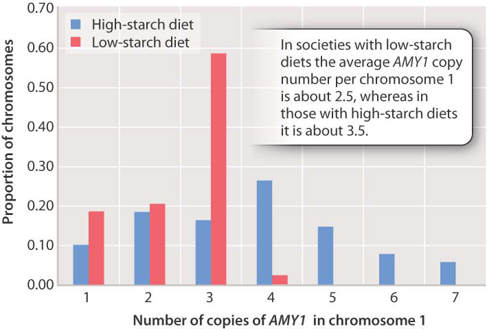
Some CNVs occur in noncoding regions, but others consist of genes that are present in multiple tandem copies along the chromosome. An example is the human gene AMY1 for the salivary-gland enzyme amylase, which aids in the digestion of starch. This gene is located in chromosome 1, and the AMY1 copy number differs from one chromosome 1 to the next. Fig. 15.10 shows the distribution of AMY1 copy number along chromosome 1 in two groups of people: societies with a long history of a high-starch diet, and societies with a long history of a low-starch diet. There is a clear tendency for chromosomes from the latter group to have fewer copies of AMY1 than those from the former group. On average, a chromosome 1 from the low-starch group has a copy number of about 2.5, whereas one from the high-starch group has an average of about 3.5. Because each individual has two copies of chromosome 1, this difference means that the average individual in the low-starch group has about 5 copies of AMY1, whereas the average individual in the high-starch group has about 7 copies. A plausible hypothesis is that extra copies were selected in groups with a high-starch diet because of the advantage extra copies conferred in digesting starch.

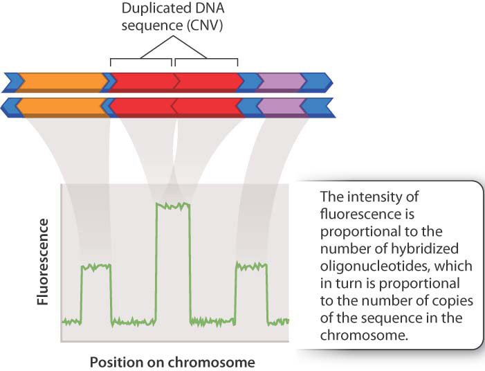
The detection of CNV is based on the relative intensity of hybridization of spots in a DNA microarray. Recall that each tiny spot on a DNA microarray holds millions of identical copies of a particular oligonucleotide sequence. In this case, the researcher chooses oligonucleotides in regions of the genome of interest, where CNV is likely. The greater the number of copies of a sequence in the genome, the more hybridization will occur when total genomic DNA is hybridized with complementary oligonucleotides on the microarray. Extra copies of a region result in greater intensity of fluorescence, and missing copies result in decreased fluorescence compared to the level of fluorescence observed for single-copy regions (Fig. 15.11).

Figure 15.11: CNV genotyping. Copy-number variation can be detected by the intensity of hybridization on a dna microarray.