21.2 MEASURING GENETIC VARIATION
Mutations, whether harmful, neutral, or advantageous, are sources of genetic variation. The goal of population genetics is to make inferences about the evolutionary process from patterns of genetic variation in nature. The raw information for this comes from the rates of occurrence of alleles in populations, or allele frequencies.
21.2.1 To understand patterns of genetic variation, we require information about allele frequencies.
The allele frequency of an allele x is simply the number of x’s present in the population divided by the total number of alleles. Consider, for example, pea color in Mendel’s pea plants. In Chapter 16, we discussed how pea color (yellow or green) results from variation at a single gene. Two alleles of this gene are the dominant A (yellow) allele and the recessive a (green) allele. AA homozygotes and Aa heterozygotes produce yellow peas, and aa homozygotes produce green peas. Imagine that in a population every pea plant produces green peas, meaning that only one allele, a, is present: The allele frequency of a is 100%, whereas the allele frequency of A is 0%. When a population exhibits only one allele at a particular gene, we say that the population is fixed for that allele.
Now consider another population of 100 pea plants with genotype frequencies of 50% aa, 25% Aa, and 25% AA. (A genotype frequency is the proportion in a population of each genotype at a particular gene or set of genes.) These genotype frequencies give us 50 green-pea pea plants (aa), 25 yellow-pea heterozygotes (Aa), and 25 yellow-pea homozygotes (AA). What is the allele frequency of a in this population? Each of the 50 aa homozygotes has two a alleles and each of the 25 heterozygotes has one a allele. Of course, there are no a alleles in AA homozygotes. The total number of a alleles is thus (2 × 50) + 25 = 125. To determine the allele frequency of a, we divide the number of a alleles by the total number of alleles in the population, 200 (because each pea plant is diploid, meaning that it has two alleles):  Because we are dealing with only two alleles in this example, the allele frequency of A is 100% −62.5% = 37.5%
Thus, the allele frequencies of A and a provide a measure of genetic variation at one gene in a given population. In this example, we were given the genotype frequencies, and from this information we determined the allele frequencies. But how are genotype and allele frequencies measured? We consider three ways to measure genotype and allele frequencies in populations: observable traits, gel electrophoresis, and DNA sequencing.
Question Quick Check 1
G43PKgMA3UsfsXfiJLkzU1qoLJLQvvuqq9HJYZkLPp+bo/QzoO5fGb1YMMV3TADicdzwOUetE9xOj7g94ByRVuPSncVMzxoG1/itP9W6yQBVhTqbOKJqboKaP+c00zzzC14qgt41/qN4EeeBoBSmxG+aYuTEsPMQfWiEu+UGMa6C3pIvcqwrOdbjGxjXQkXC9u6Xv/vBwkWq0asslWHrhPt/abbmuKYZ31CezrCdpUwtP5G4/VGiMBQMOK5LvFVs3sMBAB3NabIOBnt+zCLvoEl/caIwEYEuBucdlKQZZvYMAzCF6FsiDy2+3dPfMvAIEpXLFo17pGJwLLwl1Ie/EXEkzXeb7d7I34/PCVRjlEDlH0Mx/ZkG0cmRni0aD352y7ifW2/zsXjMgJao+prA+abMy+c=The allele frequency of a was calculated as follows:
frequency (a) = [2 x (number aa) + 1 × (number Aa) ] / [2 × (total number)]
This equation can be rewritten as
frequency (a) = [(number aa) + ½ × (number Aa)] / (total number)
Note that
number aa / total number = freqency(aa)
and
½ × (number Aa) / total number = ½ frequency(Aa)
Therefore,
frequency(a) = frequency(aa) + ½ frequency(Aa)
Stated in words, the frequency of allele a equals the frequency of aa homozygotes plus half the frequency of Aa heterozygotes. Because we were given genotype frequencies (50% aa, 25% Aa, and 25% AA), we can simply substitute into the preceding equation to solve for the frequency of a:
0.50 + ½(0.25) = 0.625, or 62.5%
By similar logic,
frequency(A) = frequency(AA) + ½ frequency(Aa)
which equals
0.25 + ½(0.25) = 0.375, or 37.5%
These equations are very useful for determining allele frequencies directly from genotype frequencies.
21-4
21.2.2 Early population geneticists relied on observable traits to measure variation.
It would be a simple matter to measure genetic variation in a population if we could use observable traits. Then we could simply count the individuals displaying variant forms of a trait and have a measure of the variation of that trait’s gene. However, as we saw in Chapter 18, this approach can work only rarely for two important reasons. First, many traits are encoded by a large number of genes. In these cases, it is difficult, if not impossible, to make direct inferences from a phenotype to the underlying genotype. Even apparently straightforward traits often prove to have a complicated genetic basis. For instance, human skin color is determined by at least six different genes. Second, the phenotype is a product of both the genotype and the environment.
Until the 1960s, there was only one workable solution: to limit population genetics to the study of phenotypes that are encoded by a single gene. As these are few, the number of genes that population geneticists could study was extremely small. Human blood groups, including the ABO system, provided an early example of a trait encoded by a single gene with multiple alleles. At this gene, there are three alleles in the population—A, B, and O—and therefore six possible genotypes, which result in four different phenotypes (Table 21.1).
| Table 21.1: The ABO blood system | |
|---|---|
| PHENOTYPE | GENOTYPE |
| A | AA or AO |
| B | BB or BO |
| AB | AB |
| O | OO |
Other instances in which phenotypic variation can be readily correlated with genotype include certain markings in invertebrates. For example, the coloring of the two-spot ladybug Adalia bipunctata is controlled by a single gene (Fig. 21.3). However, the genetic basis of most traits is not so simple.

21.2.3 Gel electrophoresis facilitates the detection of genetic variation.
Single-gene variation became much easier to detect in the 1960s with the application of gel electrophoresis. In Chapter 12, we saw how gel electrophoresis separates segments of DNA according to their size. Before DNA technologies were developed, the same basic process was applied to proteins to separate them according to their electrical charge and their size. In gel electrophoresis, the proteins being studied migrate through a gel when an electrical charge is applied, creating an electrical field. The rate at which the proteins move from one end of the gel to the other is determined by their charge and their size. Proteins with more negatively charged amino acids migrate more rapidly toward the positively charged end, and vice versa.
Early studies of protein electrophoresis focused on enzymes that catalyze reactions that can be induced to produce a dye when the substrate for the enzyme is added. If we add some of the substrate, we can see the locations of the proteins in the gel. Fig. 21.4 shows this sort of experiment. Material from different individuals is loaded in each lane of the gel. One individual, a homozygote for a particular protein sequence, produces a single band on the gel. A heterozygote for two differently charged alleles produces two bands. So the bands in the gel can provide a visual picture of genetic variation.
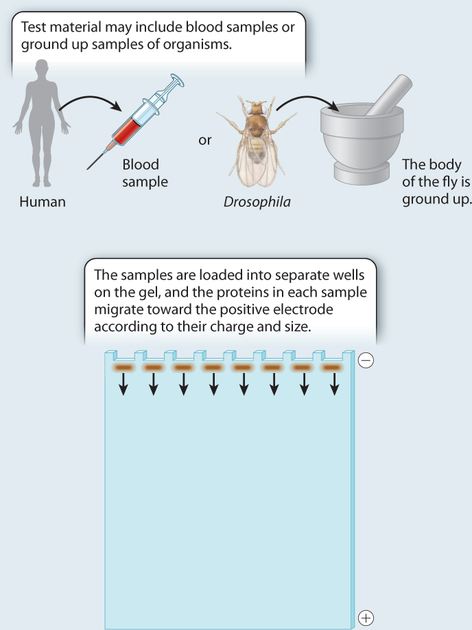
FIG. 21.4: How is genetic variation measured?
BACKGROUND The introduction of protein gel electrophoresis in 1966 gave researchers the opportunity to identify differences in amino acid sequence in proteins both among individuals and, in the case of heterozygotes, within individuals. Proteins with different amino acid sequences run at different rates through a gel in an electric field. Often, a single amino acid difference is enough to affect the mobility of a protein in a gel.
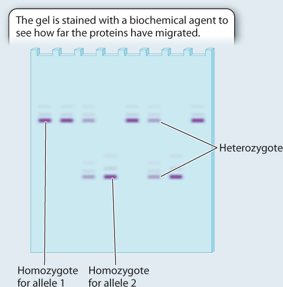
METHOD Starting with crude tissue—the whole body of a fruit fly, or a blood sample from a human—we load the material on a gel, and turn on the current. The rate at which a protein migrates depends on its size and charge, both of which may be affected by its amino acid sequence. To visualize the protein at the end of the gel run, we use a biochemical indicator that produces a stain when the protein of interest is active. The result is a series of bands on the gel.
RESULTS The genotypes of eight individuals for a gene with two alleles are analyzed. Four are allele 1 homozygotes; two are allele 2 homozygotes; and two are heterozygotes. Note that the heterozygotes do not stain as strongly on the gel because each band has half the intensity of the single band in the homozygote. We can measure the allele frequencies simply by counting the alleles. Each homozygote has two of the same allele, and each heterozygote has one of each.
Total number of alleles in the population = 8 × 2 = 16
Number of allele 1 in the population = 2 × (number of allele 1 homozygotes) + (number of heterozygotes) = 8 + 2 = 10
Frequency of allele 
Number of allele 2 in the population = 2 × (number of allele 2 homozygotes) + (number of heterozygotes) = 4 + 2 = 6
Frequency of allele 
Note that the two allele frequencies add to 1.
CONCLUSION We now have a profile of genetic variation at this gene for these individuals. Population genetics involves comparing data such as these with data collected from other populations to determine the forces shaping patterns of genetic variation.
FOLLOW-UP WORK This technique is seldom used these days because it is easy now to recover much more detailed genetic information about genetic variation from DNA sequencing.
SOURCE Lewontin, R. C., and J. L. Hubby. 1966. “A Molecular Approach to the Study of Genic heterozygosity in natural populations. II. Amount of variation and degree of heterozygosity in natural populations of Drosophila pseudoobscura.” Genetics 54:595–609.
21.2.4 DNA sequencing is the gold standard for measuring genetic variation.
Protein gel electrophoresis was a significant leap forward in our ability to detect genetic variation, but even this technique had significant limitations. We could only study enzymes because we needed to be able to stain specifically for enzyme activity, and we could only detect mutations that resulted in amino acid substitutions that changed a protein’s mobility in the gel. Only with DNA sequencing did we finally have an unambiguous means of detecting all genetic variation in a stretch of DNA, whether in a coding region or not. The variations studied by modern population geneticists are differences in DNA sequence, such as a T rather than a G at a specified nucleotide position in a particular gene.
Calculating allele frequencies, then, simply involves collecting a population sample and counting the number of occurrences of a given mutation. Take the A-or-G mutation at a specific nucleotide position in the fruit fly Alcohol dehydrogenase (Adh) gene. We can sequence the gene from 50 individual flies. We will then have 100 gene sequences from these diploid individuals. We find 70 sequences have an A and 30 have a G at a given position. Therefore, the allele frequency of A is = 0.7 and the allele frequency of G is 0.3. In general, in a sample of n diploid individuals, the allele frequency is the number of occurrences of that allele divided by twice the number of individuals.
21-5
21-6