Chapter 1. Working With Data 24.8
Working with Data: HOW DO WE KNOW? Fig. 24.8
Fig. 24.8 describes Rebecca Cann’s studies using mitochondrial DNA to map relationships among different populations of humans. Answer the questions after the figure to practice interpreting data and understanding experimental design. Some of these questions refer to concepts that are explained in the following two brief data analysis primers from a set of four available on LaunchPad:
- Experimental Design
- Data and Data Presentation
You can find these primers by clicking on the button labeled “Resources” in the menu at the upper right on your main LaunchPad page. Within the following questions, click on “Primer Section” to read the relevant section from these primers. Click on “Key Terms” to see pop-up definitions of boldfaced terms.
HOW DO WE KNOW?
FIG. 24.8: When and where did the most recent common ancestor of all living humans live?
BACKGROUND With the availability of DNA sequence analysis tools, it became possible to investigate human prehistory by comparing the DNA of living people from different populations.
HYPOTHESIS The multiregional hypothesis of human origins suggests that our most recent common ancestor was living at the time Homo ergaster populations first left Africa, about 2 million years ago.
METHOD Rebecca Cann compared mitochondrial DNA (mtDNA) sequences from 147 people from around the world. This approach required a substantial amount of mtDNA from each individual, which she acquired by collecting placentas from women after childbirth. Instead of sequencing the mtDNA, Cann inferred differences among sequences by digesting the mtDNA with different restriction enzymes, each of which cuts DNA at a specific sequence (Chapter 12). If the sequence is present, the enzyme cuts. If any base in the recognition site of the restriction enzyme has changed in an individual, the enzyme does not cut. The resulting fragments were then separated using gel electrophoresis. By using 12 different enzymes, Cann was able to assay a reasonable proportion of all the mtDNA sequence variation present in the sample.
Here, we see a sample dataset for four people and a chimpanzee. There are seven varying restriction sites:
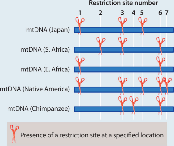
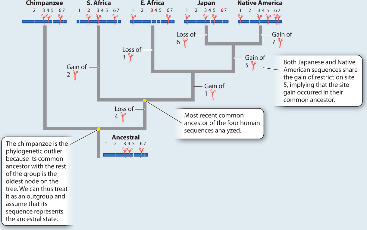
ANALYSIS The data were converted into a family tree by using shared derived characters, described in Chapter 23. By mapping the pattern of changes in this way, the phylogenetic relationships of the mtDNA sequences can be reconstructed. For example, the derived “cut” state at restriction site 1 shared by the East African, Japanese, and Native American sequences implies that the three groups had a common ancestor in which the mutation that created the new restriction site occurred.
RESULTS AND CONCLUSION A simplified version of Cann’s phylogenetic tree based on mtDNA is shown below. Modern humans arose relatively recently in Africa, and their most common ancestor lived about 200,000 years ago. The multiregional hypothesis is rejected. Also, the data revealed that all non-Africans derive from within the African family tree, implying that H. sapiens left Africa relatively recently. The Cann study gave rise to the out-of-Africa theory of human origins.
FOLLOW-UP WORK This study set the stage for an explosion in genetic studies of human prehistory that used the same approach of comparing sequences in order to identify migration patterns. Today, with molecular tools vastly more powerful than those available to Cann, studies of the distribution of genetic variation are giving us a detailed pattern, even on relatively local scales, of demographic events.
SOURCE Cann, R. L., M. Stoneking, and A. C. Wilson. 1987. “Mitochondrial DNA and Human Evolution.” Nature 325:31–36.
Question
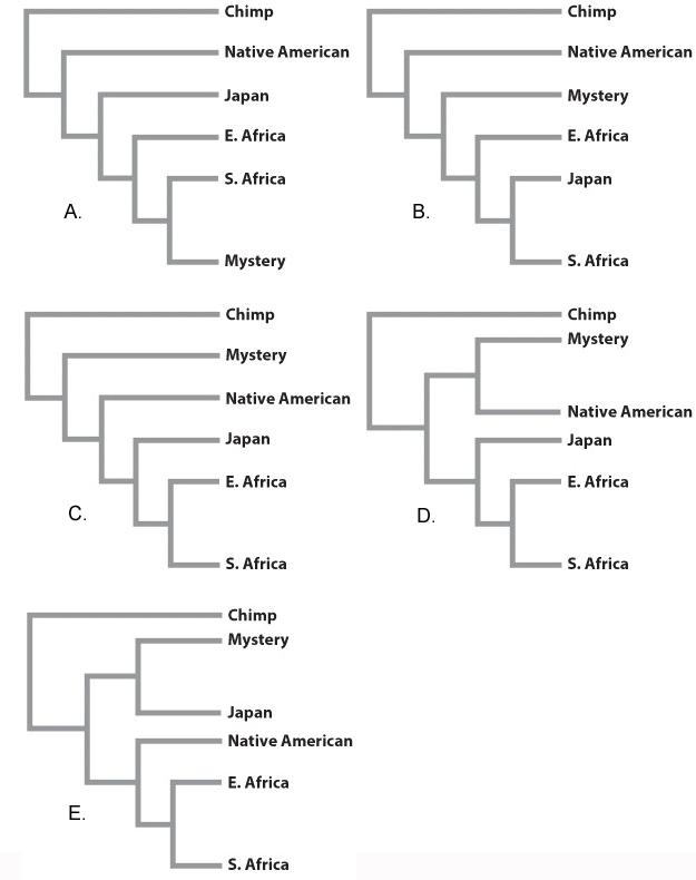
“Found Adrift!” scream the headlines. Aboard a primitive raft in the South Indian Ocean, an extraordinary new life form is found. It’s definitely humanlike, but where does it fit on the human phylogeny?
Dubbed “Mystery,” we add its DNA to our data table in Fig 24.8:
Where should it lie on the phylogeny?
Question
pwoAHmvrM1k5YgBap7qHfDj/trCmyXIlZ4tXRaeO737cZs6+wBz6IXz3feIVd2YLDx6SfiGtDf+WdeFy2XhS2CymJKNCj6rBOlMj2Gah1Sd+cyOxGROHkmXV9mu2HR2jW023hgvxfA19Ssrrd0T9VpTmV/hFx9rLO7V5wOQpBwJDx4Pp1qaWtWnooOeRkRzCz9cFC9RF+br2+Hzr0UHd2ti0eecTf/FruQ1lZBM0UJea7Uce+e5/J00zPnoxmOs+nPSP9VTtwJaOY+r2K8jfXolkQI1cTtZu+hrfZLe7Q9GfOmzhEI8pOtZZoWdV99F0jyOCOFk1fdxkgbbZHlXBdaiMjlXdP+Y824ZaVLtn4TyO4lTWYEHOvOS+NX8GeeuOqnIeffsVPPK6wKLCCYh648IchgHaD4EINqvw7orU/40BvTgxlvKCoMR4WA4JsuXaTFB4oSF7XP8c3PjDTQZPDJbhYd3jmIlQOqRURlZ2jctxj9O38yd7V7FU/oc37A/9d/XiRNF1lQAsIDtr2EhRXhMPMpOmmYFXMqOoF3GwCYpGxfBRSeGJ2zvhmf8yvNEsKt38ZfYUmKtDql9GeFpMYTCY+d0iMMQroTQtqgcYJMh44HWlGu6QyB0DYCKo972h91rD/dXObqTaEjmiR94In06DR2ZIgH03Mcx22QGZl4Arx3GTUO019ptvR9iSnNg/5lLBTtIr5Yq8SEfT/ie+sR115NWLe1eI2MW1eXwZNZ4iiU0Nk5VXmh3H4iGvXDEhSP8g6+92/8lLCdKzniV0bV6ZL4Lrph+GoQKqzuOKd/IfAhipagY3b7r74yGEmhXI/KdtVvXLUbVha+CNx05neiWMcpjPUH685uHelCdM9RNhN8A2jfhWx/Tfq+bW6R/pLyry6qnbUzgMFmBtcLMbWY6Xqwoopdeplo5eKvD/NBz5vGwAU6dhoR2hEckLJL1jAi6R/jg1OjNT+jdVmxpLlOqsmtefZyVUJrFHSo3TJzHej56XEqywWpysdZkMLtPLtVEUFcwUZZCd6np6WiqJxDC+1U4=Question
QV0Wl0Q/w8Yn83EuKw0dbFWyFksbejcQFZyG7op3zefLgIlIm9ky3NpimdqRtcHDeVSMi5wtyUg+B6T2QVAMX8JuHwiEi3nXJMDKvm1EYDguOF5d+89VKAepm4OGHhVaXhsLqUI4X+qafCVfMgcvUg0yGRU1/vxloP2O5bqEThg5orNHTCPjkyskCDgFIrXoeQG7y03r8Ou2F6rqBZ3gxPjUqH23LHXICI/8UFsBZDQt71JYSGkKdOrzNNCIEcLhNXLL3icNnJBsQI0pH4z8kn0FKpTngDVzbzQaXhSPvPI9UHZq48m7OxAbA/ZJ6uPtF+cQhsFitE3Od6wBJlaqniF3EmYAE+Z/K1JuqQAPzvw7PbLVa8PF35lxX04tJ9aNK2VF99Qay4lt4TwMUkIhFfy68Gqb8kbYxayo59mM9+ERL9bNFupLyz/VtXSzlYNbCK4SlrWoc+wym45Cp5CwcUQ5PqBNOJ3d+BxeYAJxkmwqeu944JS4XkOz0ltyeWCXYzKtDO251gMmyvP4RoeEI2CQKJiQPw/DIAxoHNq/393LEg/3QCeSRg==Question
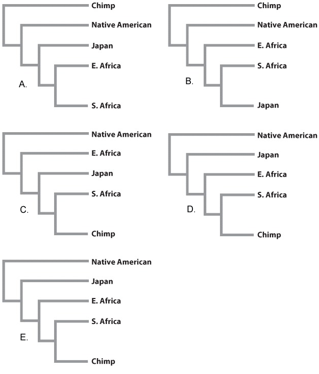
Imagine, in an alternative universe, that our species originated in North America (the Native American population), rather than Africa. Given the same set of samples as in Fig 24.8, what is the most likely phylogeny?
Question
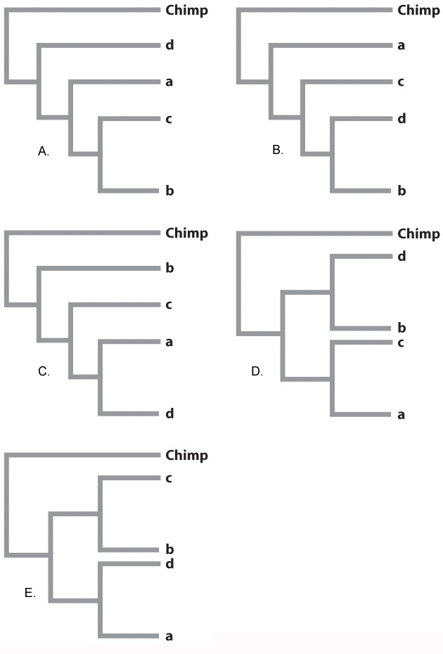
Here is some mitochondrial DNA sequence data from a study of a representative individual from each of several different human groups and a chimpanzee. Seven hundred base pairs were sequenced in total. Only the nucleotide sites that vary among the groups are represented in the table (for example, positions 1–17 are identical for the chimpanzee and all the human groups).
| DNA position | 18 | 38 | 112 | 118 | 156 | 231 | 244 | 274 | 319 | 487 | 493 | 512 | 533 | 619 |
| Chimp | T | G | G | G | A | C | G | C | G | C | T | A | G | C |
| Group a | A | A | A | G | A | C | T | T | G | T | T | A | T | C |
| Group b | A | G | G | T | C | C | T | C | G | T | C | G | T | C |
| Group c | A | G | A | G | A | G | T | T | G | T | T | A | T | T |
| Group d | A | G | G | G | C | C | T | C | A | T | T | G | T | C |
Which of the phylogenies below best represents the relationships among chimps and Groups a through d, based on the data in the table?
Question
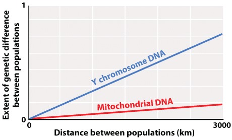
Mitochondrial DNA (mtDNA) is maternally inherited and Y-chromosome DNA is paternally inherited. In a new study, we sample multiple populations around the world for both Y-chromosome DNA and mtDNA and, through DNA sequencing, assess how genetically similar they are to each other using a measure of genetic difference in which 0 signifies genetically identical populations and 1 represents completely genetically distinct populations. We plot our data and generate regression lines as follows:
Question
gEDllVoGY6QZgkb8unlOZ1wjq6UyN0VzoZywzJ6g6lEiFOFE7QSIhJuRzXr/q9pzVKfInyNjo7L/nE6teq0IzyB1EVkai4izPwkg30vSLdo582nBPxqVB1wVbOV1rL4Yu/v7YFX7riWFPXiIPjPGvSel/G5h9Zzk6sGWsqGsYg0YGnRYLjZ0lWpr5dnOQneskLm5X5RG2xBc2ruop1F2+uu/A/Y+LsPsvKTmTicgmpEh/RQCLI1cB7EutG263l4o1aMyqbr8AYD8ymxa0Vwb7fch5mL1pYUmw7lgOX/6Ka+hIbXGa3VgqYr2FRWFjJLRUSKv8F5vYxwgmWvyB6FEolB/4kmHqoXPxGnD4msgOZreSzyP78wVbTIpFddHSv01Txsqd0vGH941uQn9UWlRVzGWq8Xehf5wKVWTUjNC8i3iFgJTPyjo9cqUwlc7a3Lp7JRMGn/VM9b34n4BTOCkbJOyf+HsSZCP/xBB7Nz84zwggp77GoJXP9UTc+4z+a7KFUnX84X5MNgVnLmLcRoqRjL9ccfeAGTT4BX+JlO15CT72CrraBM6+SQ+QVpOoIevZgObZdjbaNVtj1NujqYV2aD4LkVb5w+FofGH9U8Oehzr5BYk7S/vqm4XN+uOm2TKD8444ErogzIVZDI8PoFrG/0R+ruaybrOkkcODkdsvrqZ++LknoV6gzVXOPO7ZE1VF9YtOxF2NS019b8bcif9iwxGnIcOW4oK51zirO4YEnD1npq8HVgifsFq9YphliXNYcqjmg9L1EBuYrTAzDH+3RqRR+tE4xdTY1g0Jz3H1kC5rFWNC12MLHPQLPZpgejqXqFiHZ3geJJsVjC1/F4T1xSLBHQrowo1FPmjZhK5wjK/t7DtfqsWQ/Yx4Ng6sKMf7xTybWrzIHDOb3PVjc3r28GcMEypgJSI1H/MTrmzWsbKCyxaOl3rrZFEU84+pJtTpITIaOGiKjrspmgCuu7hIdneN1HxSfFlGTDp7TDeyP6zZJlgoie6wYqSBJ+2yiTDNBOJivdCVTi0dnhcN2lXDj+neenHf0mf1vUUyIHa5lUV2b3CJNJmH8hoht5EBeBrr/jGizM8SIjkTRDCci1wXDtCCAY35qHgdDi9SHDUGHl3S0PScuC9CmTeJPH9r+TlZbEVKZf47/M=| regression coefficient | The slope of a straight line (such as a regression line) relating values of y to those of x. |
Statistics
Correlation and Regression
Biologists often are also interested in the relation between two different measurements, such as height and weight or number of species on an island versus the size of the island. Such data are often depicted as a scatter plot (Figure 5), in which the magnitude of one variable is plotted along the x-axis and the other along the y-axis, each point representing one paired observation.
Figure 5A is the sort of data that would correspond to fingerprint ridge count (the number of raised skin ridges lying between two reference points in each fingerprint). While the data show some scatter, the overall trend is evident. There is a very strong association between the average fingerprint ridge count of parents and that of their offspring. The strength of association between two variables can be measured by the correlation coefficient, which theoretically ranges between +1 and –1. A correlation coefficient of +1 means a perfect positive relation (as one variable increases, the other increases proportionally), and a correlation coefficient of –1 implies a perfect negative relation (as one variable increases, the other decreases proportionally). Correlation coefficients of +1 or –1 are rarely observed in real data. In the case of fingerprint ridge count, the correlation coefficient is 0.9, which implies that the average fingerprint ridge count of offspring is almost (but not quite) equal to that of the parents. For a complex trait, this is a remarkably strong correlation.
Figure 5B represents data that would correspond to adult height. The data exhibit greater scatter than in Figure 5A; however, there is still a fairly strong resemblance between parents and offspring. The correlation coefficient in this case is 0.5. This value means that, on average, the offspring height is approximately halfway between that of the average of the parents and the average of the population as a whole.
The illustrations in Figure 5A and 5B also emphasize one limitation of the correlation coefficient. The correlation coefficient measures the strength of a straight-line (linear) relation. A nonlinear relation (one curving upward or downward) between two variables could be quite strong, but the data might still show a weak correlation.
Each of the straight lines in Figure 5 is a regression line or, more precisely, a regression line of y onx. Each line depicts how, on average, the variable y changes as a function of the variable x across the whole set of data. The slope of the line tells you how many units y changes, on average, for a unit change in x. A slope of +1 implies that a one-unit change in x results in a one-unit change in y, and a slope of 0 implies that the value of x has no effect on the value of y. The slope of a straight line relating values of y to those of x is known as the regression coefficient.