Chapter 1. Working With Data 7.11
Working with Data: HOW DO WE KNOW? Fig. 7.11
Fig. 7.11 describes experiments linking a proton gradient to the synthesis of ATP. Answer the questions after the figure to give you practice in interpreting data and understanding experimental design. Some of the questions refer to concepts that are explained in the following three brief data analysis primers from a set of four available on Launchpad:
- Experimental Design
- Statistics
- Scale and Approximation
You can find these primers by clicking on the button labeled “Resources” in the menu at the upper right on your main Launchpad page. Within the following questions, click on “Primer Section” to read the relevant section from these primers. Click on “Key Terms” to see pop-up definitions of boldface terms.
HOW DO WE KNOW?
FIG. 7.11: Can a proton gradient drive the synthesis of ATP?
BACKGROUND Peter Mitchell’s hypothesis that a proton gradient can drive the synthesis of ATP was proposed before experimental evidence supported it and was therefore met with skepticism. In the 1970s, biochemist Efraim Racker and his collaborator Walther Stoeckenius tested the hypothesis.
EXPERIMENT Racker and Stoeckenius built an artificial system consisting of a membrane, a bacterial proton pump activated by light, and ATP synthase.
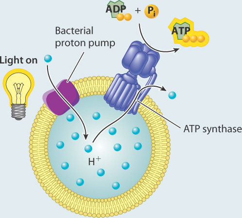
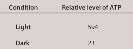
They measured the concentration of protons in the external medium and the amount of ATP produced in the presence and absence of light.
RESULTS In the presence of light, the concentration of protons increased inside the vesicles, suggesting that protons were taken up by the vesicles.

In the dark, the concentration of protons returned to the starting level. ATP was generated in the light, but not in the dark.
INTERPRETATION In the presence of light, the proton pump was activated and protons were pumped to one side of the membrane, leading to the formation of a proton gradient. The proton gradient, in turn, powered synthesis of ATP via ATP synthase.
CONCLUSION A membrane, proton gradient, and ATP synthase are sufficient to synthesize ATP. This result provided experimental evidence for Mitchell’s hypothesis.
SOURCES Mitchell, P. 1961. “Coupling of Phosphorylation to Electron and Hydrogen Transfer by a Chemiosmotic type of Mechanism.” Nature 191:144–148; Racker, E., AND W. Stoeckenius. 1974. “Reconstitution of Purple Membrane Vesicles Catalyzing Light-Driven Proton Uptake and Adenosine Triphosphate Formation.” J. Biol. Chem. 249?:?662–663.
Question
SrNkZlOWhQYp2/wi4pBpMTRCGxt84FDuz8kJ8swzo8cE01pZJ48bXYEcv/2lT9Dgq4qNrl/OW9jqOiLO6CecAFfkb9ieyl34ljpesj1vRtW+V29TuPO1tzy9KTQK0ynx65Y0NiyCmq1whVez2HK6wV0mSYO9pYj35qjMxzo8QJRz6bZNCwk2dhLbFeVLbGJJpfkrfypppe/D+0cT9eH8LIJ1+LI92Q/euImvXkOhNbOQMljHCeFUAB0nXuy+92TNZDnHrRE1b5M7JJAXpL3AcNHvuEDIJnuEd5RwsEa4mhN6HhG/0UrgEurmoi3HupCcUbzDgD+MSOlTk1gUDi5HkSGEcNf5mW7t3uTDJJ3HWlzscakCDbcejxYe8wUzXbqs9TlN45xFiR3vl0MGlvohcO6Szp8kS5uzBuouSbea1uSU24ttqntHeaTRPKxgOEmWLho7ceInYkaLFREzvmAl4o12bv/fg7q/Bfcd88xmxJkqiTnxArrjfp1aSEiCFARfT0OZIBkgXuu3Kms5av6kThHzN1bs77wdKOQxjDcXY9DtygtYDPp9zU7scI76EGZfXTRVGQ==| hypothesis | A tentative explanation for one or more observations that makes predictions that can be tested by experiments or additional observations. |
Experimental Design
Types of Hypotheses
A hypothesis, as we saw in Chapter 1, is a tentative answer to the question, an expectation of what the results might be. This might at first seem counterintuitive. Science, after all, is supposed to be unbiased, so why should you expect any particular result at all? The answer is that it helps to organize the experimental setup and interpretation of the data.
Let’s consider a simple example. We design a new medicine and hypothesize that it can be used to treat headaches. This hypothesis is not just a hunch—it is based on previous observations or experiments. For example, we might observe that the chemical structure of the medicine is similar to other drugs that we already know are used to treat headaches. If we went into the experiment with no expectation at all, it would be unclear what to measure.
A hypothesis is considered tentative because we don’t know what the answer is. The answer has to wait until we conduct the experiment and look at the data. When an experiment predicts a specific effect, as in the case of the new medicine, it is typical to also state a null hypothesis, which predicts no effect. Hypotheses are never proven, but it is possible based on statistical analysis to reject a hypothesis. When a null hypothesis is rejected, the hypothesis gains support.
Sometimes, we formulate several alternative hypotheses to answer a single question. This may be the case when researchers consider different explanations of their data. Let’s say for example that we discover a protein that represses the expression of a gene. Our question might be: How does the protein repress the expression of the gene? In this case, we might come up with several models—the protein might block transcription, it might block translation, or it might interfere with the function of the protein product of the gene. Each of these models is an alternative hypothesis, one or more of which might be correct.
Question
W/k6hqr2gf/KJXPeX3viom1XDIH4X5BMXk5o4cOboaQUgjysnbg0vVQRNmliDvVnsa3aqAAfJykoszKKpGFWC1lnbQZrPBswR6TiGGpeN29j25gSPwf5ZLJZl6OKr8nbZufc29WYO5ZCfaLY4yDgYPmJQI7JnuZvGWy9JGuEUI1UatjzZKAcTQmVpBp9k7BlqQzIUeIszoz0yyhzQhbi7z77m54hQmskO265zdJPFBHjW9iUCB+sjuWnbhwOR9urR1aBUfDWIyfNm+O2uQWSbScSkkjvdVEF51/ahCDmYxuYFphv/v0I+hj/Ud2lVVOlrGAsfBfXCjiMbEjYSdB5NbsbTvr9MgSAwlTb4eabrcg/6csK41By9n+rxp46xYtv0XtEuYJVa6c+0Y6IOSBPvtwXvLMs0aMPytF8xW8mbCEYpz48XqJJOw==| dependent variable | The effect that is being measured. |
Experimental Design
Testing Hypotheses: Variables
When performing experiments, researchers manipulate the test group differently from the control groups. This difference is known as a variable. There are two types of variables. An independent variable is the manipulation performed on the test group by the researchers. It is considered “independent” because the researchers could choose any variable they wish. The dependent variable is the effect that is being measured. It is considered “dependent” because the expectation is that it depends on the variable that was changed. In our example of the headache medicine, the independent variable is the type of medicine (new medicine, no medicine, placebo, or medicine known to be effective). The dependent variable is the presence or absence of headache following treatment.
In designing experiments, there is an additional issue to consider: the size of each of our groups. In order to draw conclusions from our data, we need to make sure that our results are valid and reproducible, and not merely the result of chance. One way to minimize the effect of chance is to include a large number of patients in each group. How many? The sample size is the number of independent data points and is determined based on probability and statistics, the subject of the next primer.
Question
GsnIB8BuIEmHURVvempHKWGkSFaQXdPoPPbydKL0kgRjrR4KZyLNqKuo3YIBtJrv8OdsCTl/P5njiLPIp7M4e0c1xl4v55nDoNhuoTKmrP8dDrXnPeRrG+ovR/KiEutl7Z3kK6VnHrqcdBGrZUq/I6yhwvUQWwLrBUWygSFLQOpWjRVZuQpk1dGtUZcaAKcOdx9YqYSCnDpe0Czd0tqu5PPGvFt12pPnCMFWG4eu4jiaQEES+xZxBP6A8OeQm5ycCn8CVD/e7gRnzWAmA6qmhrZE/5CFlA0ZA6vmXbZ1yqKKD+uauI/g3OJTx92s1Wqvtn8re9xPib402d7p5+JNZNW/kSg4gn1MK9yz7eMOpfFTgxb8quaw+6A/Lhw8Kxrf4xDUGMrNrEKVfhWlbIAZgaW8Pype7PLJ3tb3w491PN7QI4T3BQaOZhMcSTCgsAFQd2syM9RVgTMSn0XrHFWCjZMeqNVL8xmCd3OEj+oLEwj6pamS+N+LSw9umxxnJm+Itt4PeRo4ZLlfm/NxGTBL4UJguZWJ9SJRO9z7hzEGiNkMDIyEShEU2l92l2s=| independent variable | The manipulation performed on the test group by the researchers. |
Experimental Design
Testing Hypotheses: Variables
When performing experiments, researchers manipulate the test group differently from the control groups. This difference is known as a variable. There are two types of variables. An independent variable is the manipulation performed on the test group by the researchers. It is considered “independent” because the researchers could choose any variable they wish. The dependent variable is the effect that is being measured. It is considered “dependent” because the expectation is that it depends on the variable that was changed. In our example of the headache medicine, the independent variable is the type of medicine (new medicine, no medicine, placebo, or medicine known to be effective). The dependent variable is the presence or absence of headache following treatment.
In designing experiments, there is an additional issue to consider: the size of each of our groups. In order to draw conclusions from our data, we need to make sure that our results are valid and reproducible, and not merely the result of chance. One way to minimize the effect of chance is to include a large number of patients in each group. How many? The sample size is the number of independent data points and is determined based on probability and statistics, the subject of the next primer.
Question
zlHp3ylZYvgeCfCHTkSKlKz9+ODk4AexZzz/j1JvIw+wQfmlz6xSTIR6iVQidEy1lLVG8T4H9Rhc0cVenWWhjMMxHZBJrPG7Te74UYOWn0xiEdCxqX9VPs/lPvM2WKHKk6MGziLTlaNYgJ9pV5Ep9bkiBt3X7cJVORxlriLlnyyFz4fS0ZUqjCfttC0V0zpfKYneK+B/Rn+AjbxtNgXwYydVjFPhnS6ZbmhqCOucMyG1I4PiOTYOetTor/nq8QovMUKFaWg/hHivicXsKtz9og3zDCnkPpx0+xXhET+Z5K+qB832xqnAnfK/hVLGKnv+M2gpp3XO9ILn9Sco4m7v+5SRmkC+ee8TipxeLAF7cxVoIpzyp4XLHfy58hZeD6z6JQMf27rr9s2pikJaJQJshm97jVh/hKHjg2GWB/CLi04YZynOTxeyBiPzY8HxB3bkajG6np6mznijXLnPIAF470G3WKU9Oa0pW43mxuPU/pKeC8uABGsFAw==| negative control | A group in which the variable is not changed and no effect is expected. |
Experimental Design
Testing Hypotheses: Controls
Hypotheses can be tested in various ways. One way is through additional observations. There are a large number of endemic species on the Galápagos Islands. We might ask why and hypothesize that it has something to do with the location of the islands relative to the mainland. To test our hypothesis, we might make additional observations. We could count the number of endemic species on many different islands, calculate the size of each of these islands, and measure the distance from the nearest mainland. From these observations, we can understand the conditions that lead to endemic species on islands.
Hypotheses can also be tested through controlled experiments. In a controlled experiment, several different groups are tested simultaneously, keeping as many variables the same among them. In one group, a single variable is changed, allowing the researcher to see if that variable has an effect on the results of the experiment. This is called the test group. In another group, the variable is not changed and no effect is expected. This group is called the negative control. Finally, in a third group, a variable is introduced that has a known effect to be sure that the experiment is working properly. This group is called the positive control.
For example, going back to our example of a new medicine that might be effective against headaches, you could design an experiment in which there are three groups of patients—one group receives the medicine (the test group), one group receives no medicine (the negative control group), and one group receives a medicine that is already known to be effective against headaches (the positive control group). All of the other variables, such as age, gender, and socioeconomic background, would be similar among the three groups.
These three groups help the researchers to make sense of the data. Imagine for a moment that there was just the test group with no control groups, and the headaches went away after treatment. You might conclude that the medicine alleviates headaches. But perhaps the headaches just went away on their own. The negative control group helps you to see what would happen without the medicine so you can determine which effects in the test group are due solely to the medicine.
In some cases, researchers control not just for the medicine (one group receives medicine and one does not), but also for the act of giving a medicine. In this case, one negative control involves giving no medicine, and another involves giving a placebo, which is a sugar pill with no physiological effect. In this way, the researchers control for the potential variable of taking medication. In general, for a controlled experiment, it is important to be sure that there is only one difference between the test and control groups.
Question
hY44S//gCaaV0+ICYeNOLfeOFM2DJvwyieeyLAfcBsaSPrVahO7iKsn0ZM+jMUJGoUkcXq8d7DRJnQuFgmyxSf9vx5wHvLEiefYOLUYJOioL1RATGZQ9gXRFo3jzIjoJlkt2MzF0WpPmVoa7SYwPyMhckMzXKPa+Ch+yKby/xppdNAayHrFSATIQ/36SQL9TZFeM5alrAoMEwmom/Q1jyb+hxDHKu5eYlKXZuzrjrw7+lk/D3zWeiEd7NzGyjrp/U7JtiBCNGLpD6fZOMu9vBjx0YgjM2LEyJXnHOBHsbBRAlEHJXcC7z3Xyey/uKXbYso4pQbnaE1M7sRnRUOH43zBSjnNdK3wep/QpO48VWRe123A9uIumb7u0t/tDcrt2cq1zbqOneKNNUxBOYEp3q7zHcYWsgRZR2iobfZtnSLs=Question
L89jZlXto8+S4DvGCvazKxq7tIn2zEpwWPLsiyMWveGILqXM157Y2YOGhTdT+bJqC3yKCaVm6kZZ1uEUefkbo++k8DjGB8M2a2KKk7J51DFzgElgfxqr4TWjHlk2jYKhUMrdYBNsKa9W+RP2KT9zudip46KajrqJeO4wrnkR66KOCjUv| mean | The arithmetic average of all the measurements (all the measurements added together and the result divided by the number of measurements). |
Question
W5jMo0Z/ACqjVaFXIBZ0b0dVIuOWGNev1s43kCp5SJp+a90w3c0ExZmRFI5LX47CA0l5YrWXY6ztFPvLp94Tzvp1mU8yfdS9Gj68Z9FfEdTeKS986vDVk7Qn+LAwTfXmVTld7ZBCf1TkBCMFKbHhWGmrHgf16QR2Nt2KGgH/GTIokvENpUvo+so4zN4b+4Yl92gs0DY3uNlLSioOi+O23VNRAdU6wvMQIoHWCU9LyXEA5ThRZ6j6d9S7I/NuQJ41/V7pUsFXe+wdlIBHR+yTq65suFlE7yYyAxsfSBNPXgj0TzxipHZBzvU1dyvw+jBl/R0tnkPphmRT5Khlv76Cf9NHNIvj+OzgiDz2bPqdNoK0Z/uMAE9RdU5GqgAXYSVXGb6GDBGXzymecQcZGInDCO2E3yIr0lNK3gj1F6TUMMPrwhyi2gZltiBtiOit1hBzUB16iG/S7hZXpbw2XiCY+ttyPrw8NlDHvEc9YQ==| positive correlation | An association between variables such that as one variable increases, the other increases. |
| negative correlation | An association between variables such that as one variable increases, the other decreases. |
| bimodal distribution | A distribution with two modes (i.e., most frequently observed value). |
| normal distribution | The smooth, bell-shaped curve expected from the cumulative effects of many independent factors affecting the quantity being measured. |
Statistics
Correlation and Regression
Biologists often are also interested in the relation between two different measurements, such as height and weight or number of species on an island versus the size of the island. Such data are often depicted as a scatter plot (Figure 5), in which the magnitude of one variable is plotted along the x-axis and the other along the y-axis, each point representing one paired observation.
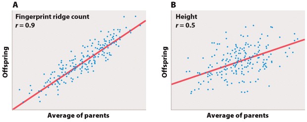
Figure 5A is the sort of data that would correspond to fingerprint ridge count (the number of raised skin ridges lying between two reference points in each fingerprint). While the data show some scatter, the overall trend is evident. There is a very strong association between the average fingerprint ridge count of parents and that of their offspring. The strength of association between two variables can be measured by the correlation coefficient, which theoretically ranges between +1 and –1. A correlation coefficient of +1 means a perfect positive relation (as one variable increases, the other increases proportionally), and a correlation coefficient of –1 implies a perfect negative relation (as one variable increases, the other decreases proportionally). Correlation coefficients of +1 or –1 are rarely observed in real data. In the case of fingerprint ridge count, the correlation coefficient is 0.9, which implies that the average fingerprint ridge count of offspring is almost (but not quite) equal to that of the parents. For a complex trait, this is a remarkably strong correlation.
Figure 5B represents data that would correspond to adult height. The data exhibit greater scatter than in Figure 5A; however, there is still a fairly strong resemblance between parents and offspring. The correlation coefficient in this case is 0.5. This value means that, on average, the offspring height is approximately halfway between that of the average of the parents and the average of the population as a whole.
The illustrations in Figure 5A and 5B also emphasize one limitation of the correlation coefficient. The correlation coefficient measures the strength of a straight-line (linear) relation. A nonlinear relation (one curving upward or downward) between two variables could be quite strong, but the data might still show a weak correlation.
Question
mM/aiybItn69KzpOyG/FF8WquxclsHpctwbkgyDToibT/M3v17r7NnU2txLI84aGYNKnbd8BkJ7RWLkOGFAG0HlgexIOOteVgCGGh5w3nOKddazZi34eK60sMvddy3vL62X6nFfDe3wnXuEPwbxSN5hOFKlR3Lpm0v6eWmrnNj1Ylb8gCQ1LR6pWnI8ZKmaIgwT/nJL75kcosuXJhN3ucFhijvBcZFhE56b+7/1fLk6ww+FgS4VCy/tFPjP7A1Ztb4GWj5wqO60yL7urnVH1epJXCCQRJ7CsWrFF95mIeqTACnZhftIOGEiGmr80Pf1w6nQxhscSuUEmn2fabAK8d9QHtWCj0xCiP+SokMOFNFmYd2XJEjbX84+ki6mMOEO3/EuUAa0dH1AvqUAwmJrniN6DSrLkP3XnT6Lu1tzjM4a4+aqXPl1Vd/Av1Rc0W3fT54KIEMxdKh7ZK5raScr9F6pgl1IpW8E/pWLjVjIpjmYViDgpVV8i/WfD2leiKgiRHuQGNwnSm1pj5bEGhTBTaZt2qEJMUQDRy4DXKqzXmp3xyU+4TgG5WLUPPFBEYv7aLX9ThM2rLjyNFeBECjGCFjeZdcEfHtXq5MBnhOZ6AazBhkRXAZwrOqNJ1NJnuIifSZpvyrzSc2U=| logarithm | The number of times a base number must be multiplied by itself to produce a specified value. |
Scale and Approximation
Logarithms
In 1614, the Scottish mathematician John Napier invented a system of calculating numbers based on exponents that he called logarithms. The logarithm of a number is the number of times a base number must be multiplied by itself to produce the value in question. From the definition, we can see a relationship to orders of magnitude, but whereas order of magnitude uses whole number exponents, logarithms can use fractions, and the base number need not be 10. For example,
16 = 101.2
so when the base is 10, the logarithm of 16 is 1.2. Moreover, the base number need not be 10. For example, the base number could be 2:
16 = 24
So in base 2, the logarithm of 16 is 4 (2 x 2 x 2 x 2 = 16). Logarithms are frequently calculated in terms of base 10, but in computer science base 2 is common, and some scientific equations use a value denoted as e (~ 2.7182818) to produce a type of logarithm called the natural logarithm. Logarithms can be obtained from tables and calculators readily available on the Internet.
Logarithms simplify calculations involving large numbers because multiplication is accomplished by adding the logarithms and division is done by subtracting one logarithm from the other. For example, 102 x 103 = 105, and 102 ÷ 103 = 10-1. In a more complicated example, 865 x 124 = 102.937 0 x 102.0934 = 105.0304 = 107,260. You can see why those logarithm tables and calculators come in handy! (In this example, we used only four significant figures in the logarithms, leading, if you calculate it out, to an approximate answer.)
Besides the utility of logarithms in making calculations – perhaps more useful in the seventeenth century than in a world of laptops and iPads – this concept is important because many relationships in nature do not scale linearly, but rather as the logarithm of one or both variables. Take the theory of island biogeography, discussed in Chapter 46. Fig. 46.18 shows the observed relationship between species richness and island size; as predicted by the theory, the number of species on an island scales with the logarithm of island area. (You might try drawing the same graph with island area on the x-axis plotted linearly.) Many well-known scales are log-based, including the pH scale used to quantify acidity, the Richter scale for earthquakes, and the decibel scale for loudness.