Chapter 2. Corn Genetics

Objectives

By the end of the period, students will be able to:

Introduction

With many genetics problems, you will be given genotype, phenotype, and possibly which genes are dominant and which are recessive. However, in most life situations, one may not know ahead of time the genotype, phenotype, or pattern of inheritance. Additionally, there are frequently challenges in scoring individuals for a particular character, as there can be a lot of individual variability.

In lab today we will use corn as our model organism.

Each lab table will have a flat of corn that was germinated recently. Each flat will be labeled with a letter. Each team of students must count the corn in each flat, and determine the cross that produced those seedlings. In some cases the crosses are a simple monohybrid cross; in other cases they are a dihybrid cross.

These flats are from a cross of unknown parents.

Your task is to deduce the phenotype and genotype of the parents for all of the flats in the room.

Here are the steps:

1. Look at the corn plants and decide on how many different phenotypes are present. There may be differences in color (green, yellow, or albino) and there may be differences in size (tall and dwarf).
2. Count and record the number of each different phenotype.
3. Look at your data and make a hypothesis about what the parental genotypes could be.
4. For your hypothesized parental genotypes, make a prediction about what the ratio of phenotypes in the offspring will be. From the ratio, calculate the expected number for each phenotype given the number of plants in each flat. (For example, if there were 200 plants and you expected a 3:1 ratio in the phenotype, you would expect the ratio of actual numbers would be 150:50.)
5. Do a Chi-square analysis. The formula for the Chi-square is on the inside front cover of your book and your TA will explain the steps. In a Chi-square analysis you are calculating a measure of how different your observed numbers are from your expected numbers given a particular hypothesis. If your Chi-square is a large number, the differences between your observed and expected values are large and your hypothesis is not supported. If you calculate a small value for the Chi-square, the difference between your observed and expected values is small and your hypothesis is supported. You will need to compare your Chi-square value to the table provided in class. You know where to look in the table by first knowing your degrees of freedom (df). In this test, degrees of freedom is the number of phenotypic classes − 1. Once you know your df, read across the row and see where your calculated Chi-square value falls. Finally, look across the top row to determine the probability that chance alone could cause the difference between observed and expected. Scientists often take a probability of 0.05 as a cutoff point for statistical significance.
6. Complete a Chi-square test for the flat on your table. As time permits, do the same for the other flats as well. Show your work. Remember that a Chi-square is always testing a specific hypothesis. Be sure to restate your hypothesis.

Example

Let’s say you have a flat of corn that has some albino individuals and some green individuals. You count them and find that there are 85 green and 15 albino individuals. You know that they all came from one set of parents. What cross could result in these numbers? Your first hypothesis may be that two heterozygotes were crossed. If that hypothesis was correct you would predict a 3:1 phenotypic ratio, or for 100 individuals, you would predict a 75:25 ratio.

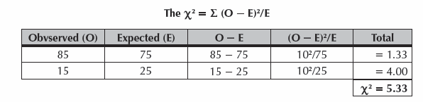
You then compare the calculated X² with X² table to see if this is significant. Degrees of freedom in this situation is the number of phenotypic classes minus 1 or

For 1 degree of freedom, the cutoff point for significance is 3.84. Our number is 5.33, which is bigger than 3.84, and so the differences are significant. That is, there is a low probability (<0.05) that chance alone would cause the differences in the observed and expected values, so something else must be causing the difference.

We reject our hypothesis.

How do you calculate the expected numbers if you don’t have 100 individuals?

Let’s say you have 250 individuals and you expect a 3:1 ratio.

In this case, 3/4 of 250 = 187.5 are expected to be green and 62.5 or 250/4 are expected to be white.