In this section, we will examine several analytical procedures that are part of everyday genetic research and are all based on the concept of independent assortment. These procedures are all used to analyze phenotypic ratios.

Genetics can work in either of two directions: (1) predicting the unknown genotypes of parents by using phenotype ratios of progeny or (2) predicting progeny phenotype ratios from parents of known genotype. The latter is an important part of genetics concerned with predicting the types of progeny that emerge from a cross and calculating their expected frequencies—in other words, their probabilities. This is useful not only in research on model organisms but also in predicting outcomes of matings in human genetics; for example in genetic counseling, people appreciate specific risk estimates. We have already examined two methods for prediction: Punnett squares and branch diagrams. Punnett squares can be used to show hereditary patterns based on one gene pair, two gene pairs, or more. Such grids are good graphic devices for representing progeny, but drawing them is time consuming. Even the 16-compartment Punnett square that we used to analyze a dihybrid cross takes a long time to write out, but, for a trihybrid cross, there are 2³, or 8, different gamete types, and the Punnett square has 64 compartments. The branch diagram (shown below) is easier to create and is adaptable for phenotypic, genotypic, or gametic proportions, as illustrated for the dihybrid A/a; B/b.

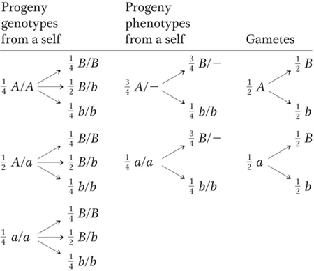
Note, however, that the “tree” of branches for genotypes is quite unwieldy even in this simple case, which uses two gene pairs, because there are 3² = 9 genotypes. For three gene pairs, there are 3³, or 27, possible genotypes. To simplify this problem, we can use a statistical approach, which constitutes a third method for calculating the probabilities (expected frequencies) of specific phenotypes or genotypes coming from a cross. The two statistical rules needed are the product rule (introduced in Chapter 2) and the sum rule, which we will now consider together.

94

The possible outcomes from rolling two dice follow the product rule because the outcome on one die is independent of the other. As an example, let us calculate the probability, p, of rolling a pair of 4’s. The probability of a 4 on one die is 1/6 because the die has six sides and only one side carries the number 4. This probability is written as follows:

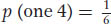
Therefore, with the use of the product rule, the probability of a 4 appearing on both dice is 1/6 × 1/6 = 1/36, which is written

Now for the sum rule:

(Note that, in the product rule, the focus is on outcomes A and B. In the sum rule, the focus is on the outcome A′ or A″.)

Dice can also be used to illustrate the sum rule. We have already calculated that the probability of two 4’s is 1/36; clearly, with the use of the same type of calculation, the probability of two 5’s will be the same, or 1/36. Now we can calculate the probability of either two 4’s or two 5’s. Because these outcomes are mutually exclusive, the sum rule can be used to tell us that the answer is 1/36 + 1/36, which is 1/18. This probability can be written as follows:

What proportion of progeny will be of a specific genotype? Now we can turn to a genetic example. Assume that we have two plants of genotypes

A/a; b/b; C/c; D/d; E/e

and

A/a; B/b; C/c; d/d; E/e

From a cross between these plants, we want to recover a progeny plant of genotype a/a; b/b; c/c; d/d; e/e (perhaps for the purpose of acting as the tester strain in a testcross). What proportion of the progeny should we expect to be of that genotype? If we assume that all the gene pairs assort independently, then we can do this calculation easily by using the product rule. The five different gene pairs are considered individually, as if five separate crosses, and then the individual probabilities of obtaining each genotype are multiplied together to arrive at the answer:

From A/a × A/a, one-fourth of the progeny will be a/a.

From b/b × B/b, half the progeny will be b/b.

From C/c × C/c, one-fourth of the progeny will be c/c.

95

From D/d × d/d, half the progeny will be d/d.

From E/e × E/e, one-fourth of the progeny will be e/e.

Therefore, the overall probability (or expected frequency) of obtaining progeny of genotype a/a; b/b; c/c; d/d; e/e will be 1/4 × 1/2 × 1/4 × 1/2 × 1/4 = 1/256. This probability calculation can be extended to predict phenotypic frequencies or gametic frequencies. Indeed, there are many other uses for this method in genetic analysis, and we will encounter some in later chapters.

How many progeny do we need to grow? To take the preceding example a step farther, suppose we need to estimate how many progeny plants need to be grown to stand a reasonable chance of obtaining the desired genotype a/a; b/b; c/c; d/d; e/e. We first calculate the proportion of progeny that is expected to be of that genotype. As just shown, we learn that we need to examine at least 256 progeny to stand an average chance of obtaining one individual plant of the desired genotype.

The probability of obtaining one “success” (a fully recessive plant) out of 256 has to be considered more carefully. This is the average probability of success. Unfortunately, if we isolated and tested 256 progeny, we would very likely have no successes at all, simply from bad luck. From a practical point of view, a more meaningful question to ask would be, What sample size do we need to be 95 percent confident that we will obtain at least one success? (Note: This 95 percent confidence value is standard in science.) The simplest way to perform this calculation is to approach it by considering the probability of complete failure—that is, the probability of obtaining no individuals of the desired genotype. In our example, for every individual isolated, the probability of its not being the desired type is 1 − (1/256) = 255/256. Extending this idea to a sample of size n, we see that the probability of no successes in a sample of n is (255/256)ⁿ. (This probability is a simple application of the product rule: 255/256 multiplied by itself n times.) Hence, the probability of obtaining at least one success is the probability of all possible outcomes (this probability is 1) minus the probability of total failure, or (255/256)ⁿ. Hence, the probability of at least one success is 1 − (255/256)ⁿ. To satisfy the 95 percent confidence level, we must put this expression equal to 0.95 (the equivalent of 95 percent).

Therefore,

1 − (255/256)ⁿ = 0.95

Solving this equation for n gives us a value of 765, the number of progeny needed to virtually guarantee success. Notice how different this number is from the naive expectation of success in 256 progeny. This type of calculation is useful in many applications in genetics and in other situations in which a successful outcome is needed from many trials.

How many distinct genotypes will a cross produce? The rules of probability can be easily used to predict the number of genotypes or phenotypes in the progeny of complex parental strains. (Such calculations are used routinely in research, in progeny analysis, and in strain building.) For example, in a self of the “tetrahybrid” A/a; B/b; C/c; D/d, there will be three genotypes for each gene pair; for example, for the first gene pair, the three genotypes will be A/a, A/A, and a/a. Because there are four gene pairs in total, there will be 3⁴ = 81 different genotypes. In a testcross of such a tetrahybrid, there will be two genotypes for each gene pair (for example, A/a and a/a) and a total of 2⁴ = 16 genotypes in the progeny. Because we are assuming that all the genes are on different chromosomes, all these testcross genotypes will occur at an equal frequency of 1/16.

96

In genetics generally, a researcher is often confronted with results that are close to an expected ratio but not identical to it. Such ratios can be from monohybrids, dihybrids, or more complex genotypes and with independence or not. But how close to an expected result is close enough? A statistical test is needed to check such numbers against expectations, and the chi-square test, or χ² test, fulfills this role.

In which experimental situations is the χ² test generally applicable? The general situation is one in which observed results are compared with those predicted by a hypothesis. In a simple genetic example, suppose you have bred a plant that you hypothesize on the basis of a preceding analysis to be a heterozygote, A/a. To test this hypothesis, you cross this heterozygote with a tester of genotype a/a and count the numbers of phenotypes with genotypes A/— and a/a in the progeny. Then, you must assess whether the numbers that you obtain constitute the expected 1:1 ratio. If there is a close match, then the hypothesis is deemed consistent with the result, whereas if there is a poor match, the hypothesis is rejected. As part of this process, a judgment has to be made about whether the observed numbers are close enough to those expected. Very close matches and blatant mismatches generally present no problem, but, inevitably, there are gray areas in which the match is not obvious.

The χ² test is simply a way of quantifying the various deviations expected by chance if a hypothesis is true. Take the preceding simple hypothesis predicting a 1:1 ratio, for example. Even if the hypothesis were true, we can only rarely expect an exact 1:1 ratio. We can model this idea with a barrelful of equal numbers of red and white marbles. If we blindly remove samples of 100 marbles, on the basis of chance we would expect samples to show small deviations such as 52 red:48 white quite commonly and to show larger deviations such as 60 red:40 white less commonly. Even 100 red marbles is a possible outcome, at a very low probability of (1/2)¹⁰⁰. However, if any result is possible at some level of probability even if the hypothesis is true, how can we ever reject a hypothesis? A general scientific convention is that a hypothesis will be rejected as false if there is a probability of less than 5 percent of observing a deviation from expectations at least as large as the one actually observed. The hypothesis might still be true, but we have to make a decision somewhere, and 5 percent is the conventional decision line. The implication is that, although results this far from expectations are expected 5 percent of the time even when the hypothesis is true, we will mistakenly reject the hypothesis in only 5 percent of cases and we are willing to take this chance of error. (This 5 percent is the converse of the 95 percent confidence level used earlier.)

Let’s look at some real data. We will test our earlier hypothesis that a plant is a heterozygote. We will let A stand for red petals and a stand for white. Scientists test a hypothesis by making predictions based on the hypothesis. In the present situation, one possibility is to predict the results of a testcross. Assume that we testcross the presumed heterozygote. On the basis of the hypothesis, Mendel’s law of equal segregation predicts that we should have 50 percent A/a and 50 percent a/a. Assume that, in reality, we obtain 120 progeny and find that 55 are red and 65 are white. These numbers differ from the precise expectations, which would have been 60 red and 60 white. The result seems a bit far off the expected ratio, which raises uncertainty; so we need to use the χ² test. We calculate χ² by using the following formula:

χ² = Σ (O – E)²/E for all classes

in which E is the expected number in a class, O is the observed number in a class, and Σ means “sum of.” The resulting value, χ², will provide a numerical value that estimates the degree of agreement between the expected (hypothesized) and observed (actual) results, with the number growing larger as the agreement increases.

97

The calculation is most simply performed by using a table:

Now we must look up this χ² value in Table 3-1, which will give us the probability value that we want. The rows in Table 3-1 list different values of degrees of freedom (df). The number of degrees of freedom is the number of independent variables in the data. In the present context, the number of independent variables is simply the number of phenotypic classes minus 1. In this case, df = 2 − 1 = 1. So we look only at the 1 df line. We see that our χ² value of 0.84 lies somewhere between the columns marked 0.5 and 0.1—in other words, between 50 percent and 10 percent. This probability value is much greater than the cutoff value of 5 percent, and so we accept the observed results as being compatible with the hypothesis.

Some important notes on the application of this test follow:

Any of the familiar Mendelian ratios considered in this chapter or in Chapter 2 can be tested by using the χ² test—for example, 3:1 (1 df), 1:2:1 (2 df), 9:3:3:1 (3 df), and 1:1:1:1 (3 df). We will return to more applications of the χ² test in Chapter 4.

Pure lines are among the essential tools of genetics. For one thing, only these fully homozygous lines will express recessive alleles, but the main need for pure lines is in the maintenance of stocks for research. The members of a pure line can be left to interbreed over time and thereby act as a constant source of the genotype for use in experiments. Hence, for most model organisms, there are international stock centers that are repositories of pure lines for use in research. Similar stock centers provide lines of plants and animals for use in agriculture.

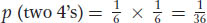
Pure lines of plants or animals are made through repeated generations of selfing. (In animals, selfing is accomplished by mating animals of identical genotype.) Selfing a monohybrid plant shows the principle at work. Suppose we start with a population of individuals that are all A/a and allow them to self. We can apply Mendel’s first law to predict that, in the next generation, there will be A/A, A/a, and a/a. Note that the heterozygosity (the proportion of heterozygotes) has halved, from 1 to . If we repeat this process of selfing for another generation, all descendants of homozygotes will be homozygous, but, again, the heterozygotes will halve their proportion to a quarter. The process is shown in the following display:

After, say, eight generations of selfing, the proportion of heterozygotes is reduced to (1/2)⁸, which is 1/256, or about 0.4 percent. Let’s look at this process in a slightly different way: we will assume that we start such a program with a genotype that is heterozygous at 256 gene pairs. If we also assume independent assortment, then, after selfing for eight generations, we would end up with an array of genotypes, each having on average only one heterozygous gene (that is, 1/256). In other words, we are well on our way to creating a number of pure lines.

Let us apply this principle to the selection of agricultural lines, the topic with which we began the chapter. We can use as our example the selection of Marquis wheat by Charles Saunders in the early part of the twentieth century. Saunders’s goal was to develop a productive wheat line that would have a shorter growing season and hence open up large areas of terrain in northern countries such as Canada and Russia for growing wheat, another of the world’s staple foods. He crossed a line having excellent grain quality called Red Fife with a line called Hard Red Calcutta, which, although its yield and quality were poor, matured 20 days earlier than Red Fife. The F₁ produced by the cross was presumably heterozygous for multiple genes controlling the wheat qualities. From this F₁, Saunders made selfings and selections that eventually led to a pure line that had the combination of favorable properties needed—good-quality grain and early maturation. This line was called Marquis. It was rapidly adopted in many parts of the world.

99

A similar approach can be applied to the rice lines with which we began the chapter. All the single-gene mutations are crossed in pairs, and then their F₁ plants are selfed or intercrossed with other F₁ plants. As a demonstration, let’s consider just four mutations, 1 through 4. A breeding program might be as follows, in which the mutant alleles and their wild-type counterparts are always listed in the same order (recall that the + sign designates wild type):

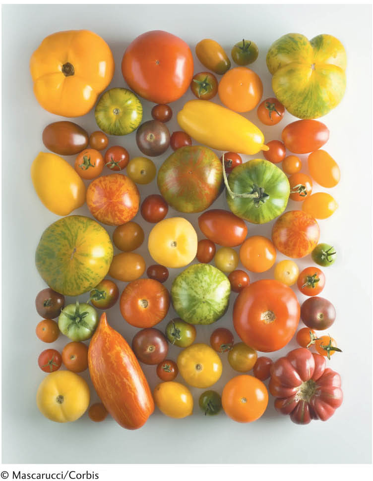
This type of breeding has been applied to many other crop species. The colorful and diverse pure lines of tomatoes used in commerce are shown in Figure 3-5.

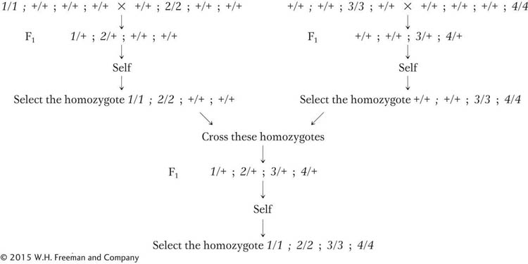
Note that, in general when a multiple heterozygote is selfed, a range of different homozygotes is produced. For example, from A/a; B/b; C/c, there are two homozygotes for each gene pair (that is, for the first gene, the homozygotes are A/A and a/a), and so there are 2³ = 8 different homozygotes possible: A/A; b/b; C/c, and a/a; B/B; c/c, and so on. Each distinct homozygote can be the start of a new pure line.

We have been considering the synthesis of superior pure lines for research and for agriculture. Pure lines are convenient in that propagation of the genotype from year to year is fairly easy. However, a large proportion of commercial seed that farmers (and gardeners) use is called hybrid seed. Curiously, in many cases in which two disparate lines of plants (and animals) are united in an F₁ hybrid (presumed heterozygote), the hybrid shows greater size and vigor than do the two contributing lines (Figure 3-6). This general superiority of multiple heterozygotes is called hybrid vigor. The molecular reasons for hybrid vigor are mostly unknown and still hotly debated, but the phenomenon is undeniable and has made large contributions to agriculture. A negative aspect of using hybrids is that, every season, the two parental lines must be grown separately and then intercrossed to make hybrid seed for sale. This process is much more inconvenient than maintaining pure lines, which requires only letting plants self; consequently, hybrid seed is more expensive than seed from pure lines.

100

From the user’s perspective, there is another negative aspect of using hybrids. After a hybrid plant has grown and produced its crop for sale, it is not realistic to keep some of the seeds that it produces and expect this seed to be equally vigorous the next year. The reason is that, when the hybrid undergoes meiosis, independent assortment of the various mixed gene pairs will form many different allelic combinations, and very few of these combinations will be that of the original hybrid. For example, the earlier described tetrahybrid, when selfed, produces 81 different genotypes, of which only a minority will be tetrahybrid. If we assume independent assortment, then, for each gene pair, selfing will produce one-half heterozygotes A/a → A/A, A/a, and a/a. Because there are four gene pairs in this tetrahybrid, the proportion of progeny that will be like the original hybrid A/a; B/b; C/c; D/d will be (1/2)⁴ = 1/16.

101