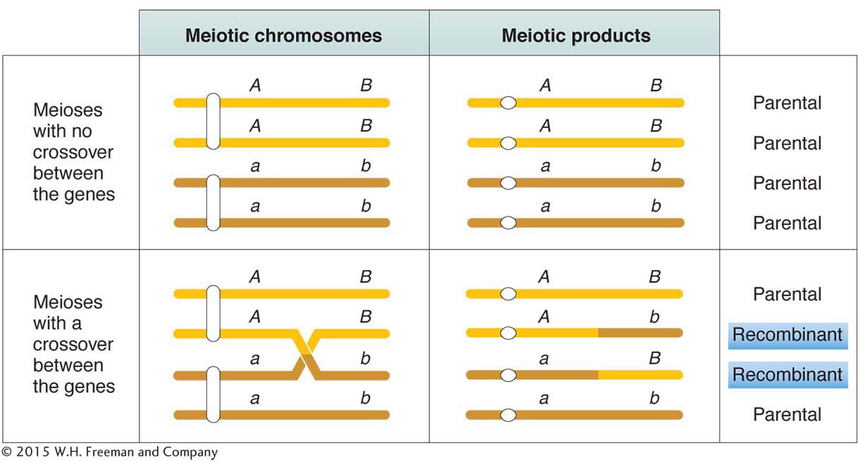
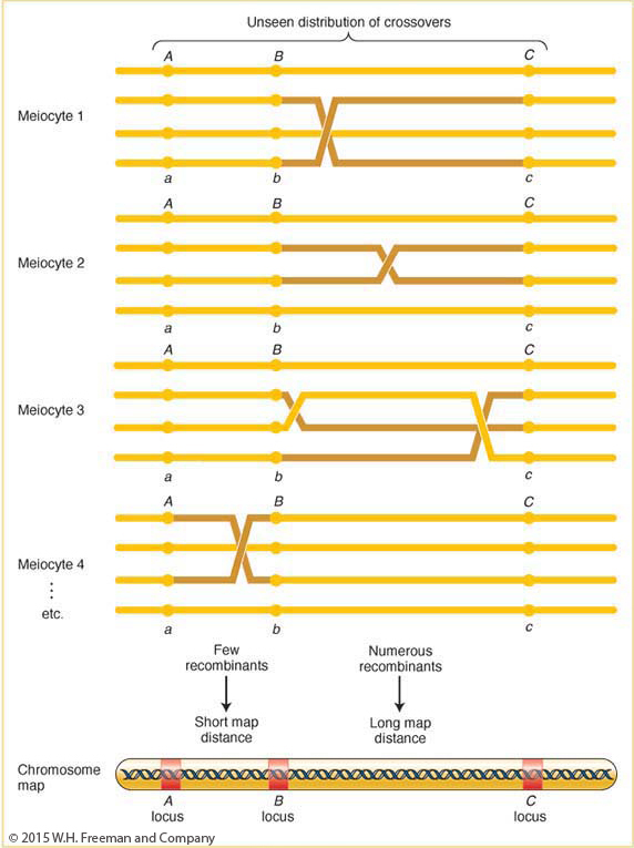
The frequency of recombinants produced by crossing over is the key to chromosome mapping. Fungal tetrad analysis has shown that, for any two specific linked genes, crossovers take place between them in some, but not all, meiocytes (Figure 4-7). The farther apart the genes are, the more likely that a crossover will take place and the higher the proportion of recombinant products will be. Thus, the proportion of recombinants is a clue to the distance separating two gene loci on a chromosome map.

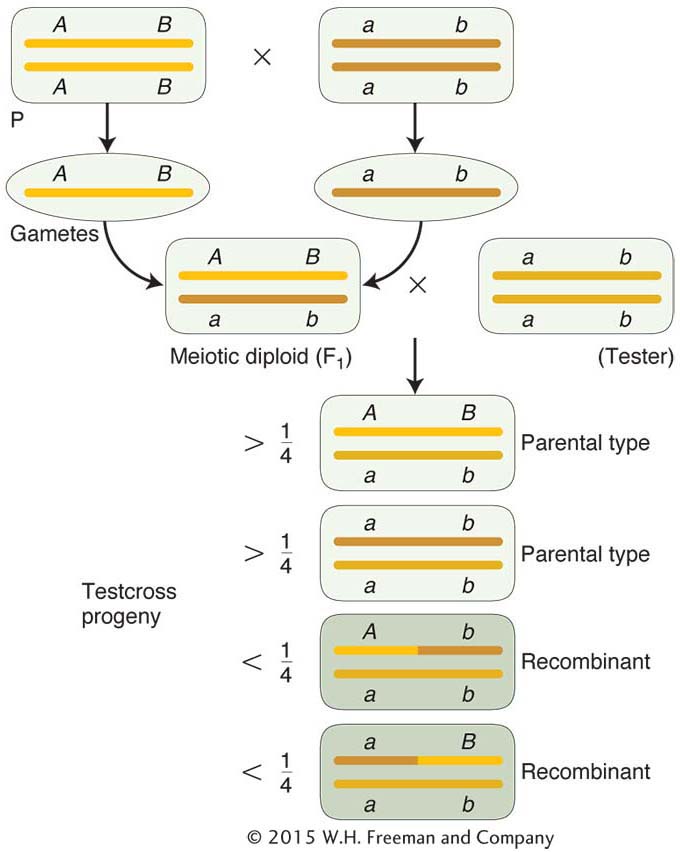
As stated earlier in regard to Morgan’s data, the recombinant frequency was significantly less than 50 percent, specifically 10.7 percent. Figure 4-8 shows the general situation for linkage in which recombinants are less than 50 percent. Recombinant frequencies for different linked genes range from 0 to 50 percent, depending on their closeness. The farther apart genes are, the more closely their recombinant frequencies approach 50 percent, and, in such cases, one cannot decide whether genes are linked or are on different chromosomes. What about recombinant frequencies greater than 50 percent? The answer is that such frequencies are never observed, as will be proved later.

136

Note in Figure 4-7 that a single crossover generates two reciprocal recombinant products, which explains why the reciprocal recombinant classes are generally approximately equal in frequency. The corollary of this point is that the two parental nonrecombinant types also must be equal in frequency, as also observed by Morgan.

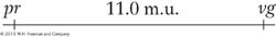
The basic method of mapping genes with the use of recombinant frequencies was devised by a student of Morgan’s. As Morgan studied more and more linked genes, he saw that the proportion of recombinant progeny varied considerably, depending on which linked genes were being studied, and he thought that such variation in recombinant frequency might somehow indicate the actual distances separating genes on the chromosomes. Morgan assigned the quantification of this process to an undergraduate student, Alfred Sturtevant, who also became one of the great geneticists. Morgan asked Sturtevant to try to make some sense of the data on crossing over between different linked genes. In one evening, Sturtevant developed a method for mapping genes that is still used today. In Sturtevant’s own words, “In the latter part of 1911, in conversation with Morgan, I suddenly realized that the variations in strength of linkage, already attributed by Morgan to differences in the spatial separation of genes, offered the possibility of determining sequences in the linear dimension of a chromosome. I went home and spent most of the night (to the neglect of my undergraduate homework) in producing the first chromosome map.” As an example of Sturtevant’s logic, consider Morgan’s testcross results with the pr and vg genes, from which he calculated a recombinant frequency of 10.7 percent. Sturtevant suggested that we can use this percentage of recombinants as a quantitative index of the linear distance between two genes on a genetic map, or linkage map, as it is sometimes called.

The basic idea here is quite simple. Imagine two specific genes positioned a certain fixed distance apart. Now imagine random crossing over along the paired homologs. In some meioses, nonsister chromatids cross over by chance in the chromosomal region between these genes; from these meioses, recombinants are produced. In other meiotic divisions, there are no crossovers between these genes; no recombinants result from these meioses. (See Figure 4-7 for a diagrammatic illustration.) Sturtevant postulated a rough proportionality: the greater the distance between the linked genes, the greater the chance of crossovers in the region between the genes and, hence, the greater the proportion of recombinants that would be produced. Thus, by determining the frequency of recombinants, we can obtain a measure of the map distance between the genes. In fact, Sturtevant defined one genetic map unit (m.u.) as that distance between genes for which 1 product of meiosis in 100 is recombinant. For example, the recombinant frequency (RF) of 10.7 percent obtained by Morgan is defined as 10.7 m.u. A map unit is sometimes referred to as a centimorgan (cM) in honor of Thomas Hunt Morgan.

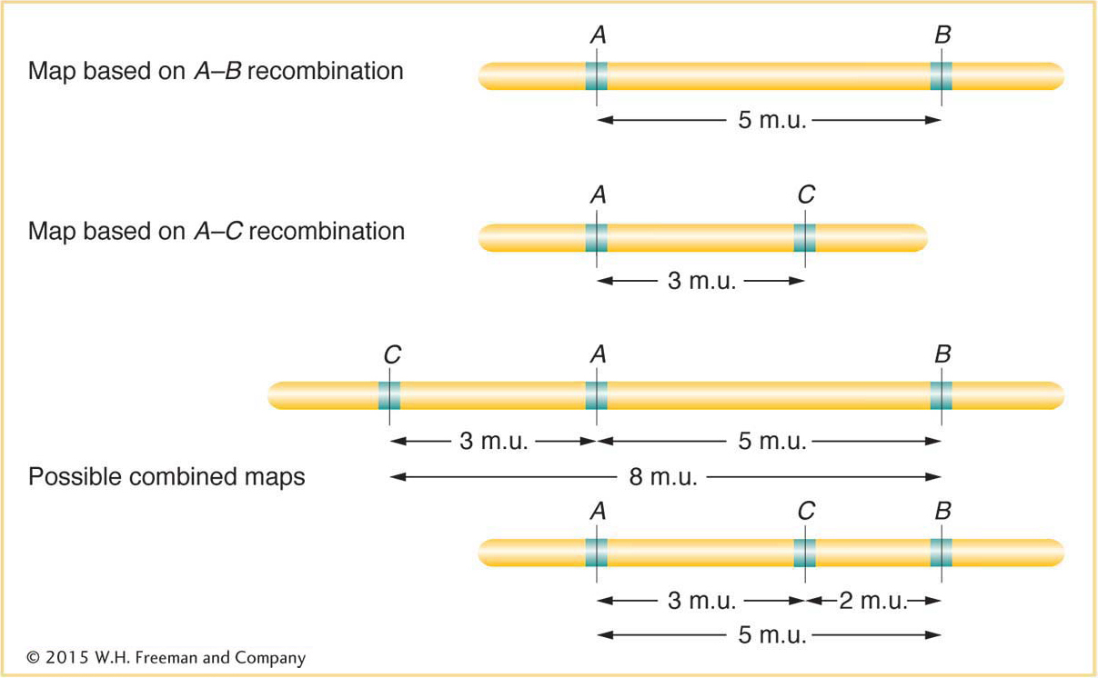
Does this method produce a linear map corresponding to chromosome linearity? Sturtevant predicted that, on a linear map, if 5 map units (5 m.u.) separate genes A and B, and 3 m.u. separate genes A and C, then the distance separating B and C should be either 8 or 2 m.u. (Figure 4-9). Sturtevant found his prediction to be the case. In other words, his analysis strongly suggested that genes are arranged in some linear order, making map distances additive. (There are some minor but not insignificant exceptions, as we will see later.) Since we now know from molecular analysis that a chromosome is a single DNA molecule with the genes arranged along it, it is no surprise for us today to learn that recombination-based maps are linear because they reflect a linear array of genes.

137

How is a map represented? As an example, in Drosophila, the locus of the eye-color gene and the locus of the wing-length gene are approximately 11 m.u. apart, as mentioned earlier. The relation is usually diagrammed in the following way:

Generally, we refer to the locus of this eye-color gene in shorthand as the “pr locus,” after the first discovered mutant allele, but we mean the place on the chromosome where any allele of this gene will be found, mutant or wild type.

As stated in Chapters 2 and 3, genetic analysis can be applied in two opposite directions. This principle is applicable to recombinant frequencies. In one direction, recombinant frequencies can be used to make maps. In the other direction, when given an established map with genetic distance in map units, we can predict the frequencies of progeny in different classes. For example, the genetic distance between the pr and vg loci in Drosophila is approximately 11 m.u. So knowing this value, we know that there will be 11 percent recombinants in the progeny from a testcross of a female dihybrid heterozygote in cis conformation (pr vg/pr⁺ vg⁺). These recombinants will consist of two reciprocal recombinants of equal frequency: thus, 5.5 percent will be pr⁺ vg⁺ and 5.5 percent will be pr⁺vg. We also know that 100 – 11 = 89 percent will be nonrecombinant in two equal classes, 44.5 percent pr⁺ vg⁺ and 44.5 percent pr vg. (Note that the tester contribution pr vg was ignored in writing out these genotypes.)

There is a strong implication that the “distance” on a linkage map is a physical distance along a chromosome, and Morgan and Sturtevant certainly intended to imply just that. But we should realize that the linkage map is a hypothetical entity constructed from a purely genetic analysis. The linkage map could have been derived without even knowing that chromosomes existed. Furthermore, at this point in our discussion, we cannot say whether the “genetic distances” calculated by means of recombinant frequencies in any way represent actual physical distances on chromosomes. However, physical mapping has shown that genetic distances are, in fact, roughly proportional to recombination-based distances. There are exceptions caused by recombination hotspots, places in the genome where crossing over takes place more frequently than usual. The presence of hotspots causes proportional expansion of some regions of the map. Recombination blocks, which have the opposite effect, also are known.

138

A summary of the way in which recombinants from crossing over are used in mapping is shown in Figure 4-10. Crossovers occur more or less randomly along the chromosome pair. In general, in longer regions, the average number of crossovers is higher and, accordingly, recombinants are more frequently obtained, translating into a longer map distance.

139

So far, we have looked at linkage in crosses of dihybrids (double heterozygotes) with doubly recessive testers. The next level of complexity is a cross of a trihybrid (triple heterozygote) with a triply recessive tester. This kind of cross, called a three-point testcross or a three-factor cross, is commonly used in linkage analysis. The goal is to deduce whether the three genes are linked and, if they are, to deduce their order and the map distances between them.

Let’s look at an example, also from Drosophila. In our example, the mutant alleles are v (vermilion eyes), cv (crossveinless, or absence of a crossvein on the wing), and ct (cut, or snipped, wing edges). The analysis is carried out by performing the following crosses:

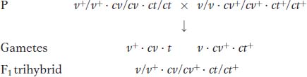
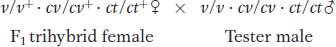
Trihybrid females are testcrossed with triple recessive males:

From any trihybrid, only 2 × 2 × 2 = 8 gamete genotypes are possible. They are the genotypes seen in the testcross progeny. The following chart shows the number of each of the eight gametic genotypes in a sample of 1448 progeny flies. The columns alongside show which genotypes are recombinant (R) for the loci taken two at a time. We must be careful in our classification of parental and recombinant types. Note that the parental input genotypes for the triple heterozygotes are v⁺ · cv · ct and v · cv + · ct⁺; any combination other than these two constitutes a recombinant.

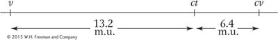
Let’s analyze the loci two at a time, starting with the v and cv loci. In other words, we look at just the first two columns under “Gametes” and cover up the third one. Because the parentals for this pair of loci are v⁺ · cv and v · cv⁺, we know that the recombinants are by definition v · cv and v⁺ · cv⁺. There are 45 + 40 + 89 + 94 = 268 of these recombinants. Of a total of 1448 flies, this number gives an RF of 18.5 percent.

140

For the v and ct loci, the recombinants are v · ct and v⁺ · ct⁺. There are 89 + 94 + 3 + 5 = 191 of these recombinants among 1448 flies, and so the RF = 13.2 percent.

For ct and cv, the recombinants are cv · ct⁺ and cv⁺ · ct. There are 45 + 40 + 3 + 5 = 93 of these recombinants among the 1448, and so the RF = 6.4 percent.

Clearly, all the loci are linked, because the RF values are all considerably less than 50 percent. Because the v and cv loci have the largest RF value, they must be farthest apart; therefore, the ct locus must lie between them. A map can be drawn as follows:

The testcross can be rewritten as follows, now that we know the linkage arrangement:

v⁺ ct cv/v ct⁺ cv⁺ × v ct cv/v ct cv

Note several important points here. First, we have deduced a gene order that is different from that used in our list of the progeny genotypes. Because the point of the exercise was to determine the linkage relation of these genes, the original listing was of necessity arbitrary; the order was simply not known before the data were analyzed. Henceforth, the genes must be written in correct order.

Second, we have definitely established that ct is between v and cv. In the diagram, we have arbitrarily placed v to the left and cv to the right, but the map could equally well be drawn with the placement of these loci inverted.

Third, note that linkage maps merely map the loci in relation to one another, with the use of standard map units. We do not know where the loci are on a chromosome—or even which specific chromosome they are on. In subsequent analyses, as more loci are mapped in relation to these three, the complete chromosome map would become “fleshed out.”

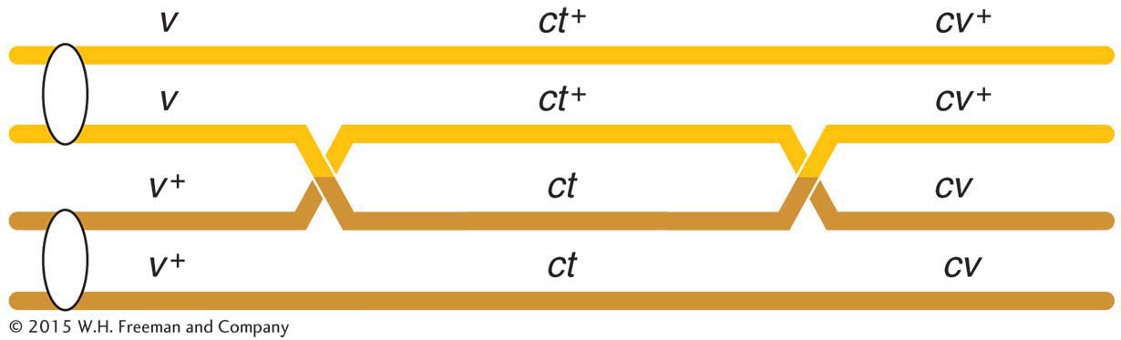
A final point to note is that the two smaller map distances, 13.2 m.u. and 6.4 m.u., add up to 19.6 m.u., which is greater than 18.5 m.u., the distance calculated for v and cv. Why? The answer to this question lies in the way in which we have treated the two rarest classes of progeny (totaling 8) with respect to the recombination of v and cv. Now that we have the map, we can see that these two rare classes are in fact double recombinants, arising from two crossovers (Figure 4-11). However, when we calculated the RF value for v and cv, we did not count the v ct cv⁺ and v⁺ ct⁺ cv genotypes; after all, with regard to v and cv, they are parental combinations (v cv⁺ and v⁺ cv). In light of our map, however, we see that this oversight led us to underestimate the distance between the v and the cv loci. Not only should we have counted the two rarest classes, we should have counted each of them twice because each represents double recombinants. Hence, we can correct the value by adding the numbers 45 + 40 + 89 + 94 + 3 + 3 + 5 + 5 = 284. Of the total of 1448, this number is exactly 19.6 percent, which is identical with the sum of the two component values. (In practice, we do not need to do this calculation, because the sum of the two shorter distances gives us the best estimate of the overall distance.)

141

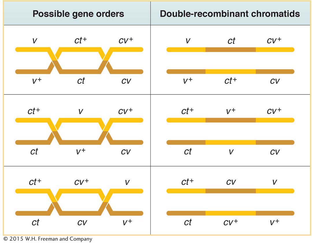
Now that we have had some experience with the three-point testcross, we can look back at the progeny listing and see that, for trihybrids of linked genes, gene order can usually be deduced by inspection, without a recombinant frequency analysis. Typically, for linked genes, we have the eight genotypes at the following frequencies:

two at high frequency

two at intermediate frequency

two at a different intermediate frequency

two rare

Only three gene orders are possible, each with a different gene in the middle position. It is generally true that the double-recombinant classes are the smallest ones, as listed last here. Only one order is compatible with the smallest classes’ having been formed by double crossovers, as shown in Figure 4-12; that is, only one order gives double recombinants of genotype v ct cv⁺ and v⁺ ct⁺ cv. A simple rule of thumb for deducing the gene in the middle is that it is the allele pair that has “flipped” position in the double-recombinant classes.

Knowing the existence of double crossovers permits us to ask questions about their possible interdependence. We can ask, Are the crossovers in adjacent chromosome regions independent events or does a crossover in one region affect the likelihood of there being a crossover in an adjacent region? The answer is that, generally, crossovers inhibit each other somewhat in an interaction called interference. Double-recombinant classes can be used to deduce the extent of this interference.

Interference can be measured in the following way. If the crossovers in the two regions are independent, we can use the product rule to predict the frequency of double recombinants: that frequency would equal the product of the recombinant frequencies in the adjacent regions. In the v-ct-cv recombination data, the v-ct RF value is 0.132 and the ct-cv value is 0.064; so, if there is no interference, double recombinants might be expected at the frequency 0.132 × 0.064 = 0.0084 (0.84 percent). In the sample of 1448 flies, 0.0084 × 1448 = 12 double recombinants are expected. But the data show that only 8 were actually observed. If this deficiency of double recombinants were consistently observed, it would show us that the two regions are not independent and suggest that the distribution of crossovers favors singles at the expense of doubles. In other words, there is some kind of interference: a crossover does reduce the probability of a crossover in an adjacent region.

142

Interference is quantified by first calculating a term called the coefficient of coincidence (c.o.c.), which is the ratio of observed to expected double recombinants. Interference (I) is defined as 1 − c.o.c. Hence,

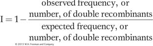
In our example,

In some regions, there are never any observed double recombinants. In these cases, c.o.c. = 0, and so I = 1 and interference is complete. Interference values anywhere between 0 and 1 are found in different regions and in different organisms.

You may have wondered why we always use heterozygous females for testcrosses in Drosophila. The explanation lies in an unusual feature of Drosophila males. When, for example, pr vg/pr⁺ vg⁺ males are crossed with pr vg/pr vg females, only pr vg/pr⁺ vg⁺ and pr vg/pr vg progeny are recovered. This result shows that there is no crossing over in Drosophila males. However, this absence of crossing over in one sex is limited to certain species; it is not the case for males of all species (or for the heterogametic sex). In other organisms, there is crossing over in XY males and in WZ females. The reason for the absence of crossing over in Drosophila males is that they have an unusual prophase I, with no synaptonemal complexes. Incidentally, there is a recombination difference between human sexes as well. Women show higher recombinant frequencies for the same autosomal loci than do men.

With the use of a reiteration of the preceding recombination-based techniques, maps have been produced of thousands of genes for which variant (mutant) phenotypes have been identified. A simple illustrative example from the tomato is shown in Figure 4-13. The tomato chromosomes are shown in Figure 4-13a, their numbering in Figure 4-13b, and recombination-based gene maps in Figure 4-13c. The chromosomes are shown as they appear under the microscope, together with chromosome maps based on linkage analysis of various allelic pairs shown with their phenotypes.

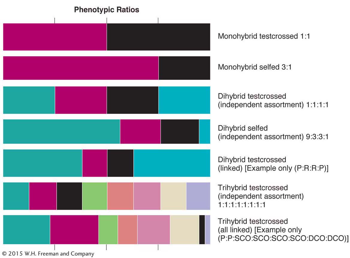
The analysis of ratios is one of the pillars of genetics. In the text so far, we have encountered many different ratios whose derivations are spread out over several chapters. Because recognizing ratios and using them in diagnosis of the genetic system under study are part of everyday genetics, let’s review the main ratios that we have covered so far. They are shown in Figure 4-14. You can read the ratios from the relative widths of the colored boxes in a row. Figure 4-14 deals with selfs and testcrosses of monohybrids, dihybrids (with independent assortment and linkage), and trihybrids (also with independent assortment and linkage of all genes). One situation not represented is a trihybrid in which only two of the three genes are linked; as an exercise, you might like to deduce the general pattern that would have to be included in such a diagram from this situation. Note that, in regard to linkage, the sizes of the classes depend on map distances. A geneticist deduces unknown genetic states in something like the following way: “a 9:3:3:1 ratio tells me that this ratio was very likely produced by a selfed dihybrid in which the genes are on different chromosomes.”

143

144