So far in this chapter we have mapped gene loci using RF values by counting visible phenotypes produced by the various alleles involved. However, there are also differences in the DNA between two chromosomes that do not produce visibly different phenotypes, either because these DNA differences are not located in genes or they are located in genes but do not alter the product protein. Such sequence differences can be thought of as molecular alleles or molecular markers. Their loci can be mapped by RF values in the same way as alleles producing visible phenotypes. Molecular markers are extremely numerous and hence are very useful as genomic landmarks that can be used to locate genes of interest.

The two main types of molecular markers used in mapping are single nucleotide polymorphisms and simple sequence length polymorphisms.

Sequencing has shown that, as expected, the genomic sequences of individuals in a species are mostly identical. For example, comparisons of the sequences of different individuals have revealed that we are about 99.9 percent identical. Almost all of the 0.1 percent difference turns out to be based on singlenucleotide differences. As an example, in one individual, a localized sequence might be

....AAGGCTCAT....

....TTCCGAGTA....

and, in another, it might be

....AAAGCTCAT....

....TTTCGAGTA....

145

Furthermore, a large proportion of these localized sequences are found to be polymorphic, meaning that both molecular “alleles” are quite common in the population. Overall, such differences between individuals are called single nucleotide polymorphisms, abbreviated as SNPs and pronounced “snips.” In humans, there are thought to be about 3 million SNPs distributed more or less randomly at a frequency of 1 in every 300 to 1000 bases.

Some of these SNPs lie within genes; many do not. In Chapter 2, we saw cases where the change in a single nucleotide pair could produce a new allele, causing a mutant phenotype. The two nucleotide pairs, wild type and mutant, are examples of a SNP. Most SNPs, though, do not produce different phenotypes, either because they do not lie in a gene or because they lie in a gene but both versions of the gene produce the same protein product.

There are two ways to detect a SNP The first is to sequence a segment of DNA in homologous chromosomes and compare the homologous segments to spot differences. A second way is possible in the case of SNPs located at a restriction enzyme’s target site: these SNPs are restriction fragment length polymorphisms (RFLPs). In such cases, there will be two RFLP “alleles,” or morphs, one of which has the restriction enzyme target and the other of which does not. The restriction enzyme will cut the DNA at the SNP containing the target and ignore the other SNP. The SNPs are then detected as different bands on an electrophoretic gel. RFLP sites can be between or within genes.

One of the surprises from molecular genomic analysis is that most genomes contain a great deal of repetitive DNA. Furthermore, there are many types of repetitive DNA. At one end of the spectrum are adjacent multiple repeats of short, simple DNA sequences. The origin of these repeats is not clear, but the feature that makes them useful is that, in different individuals, there are often different numbers of copies. Hence, these repeats are called simple sequence length polymorphisms (SSLPs). They are also sometimes called variable number tandem repeats, or VNTRs.

SSLPs commonly have multiple alleles; as many as 15 alleles have been found for an SSLP locus. As a consequence, sometimes 4 alleles (2 from each parent) can be tracked in a pedigree. Two types of SSLPs are useful in mapping and other genome analysis: minisatellite and microsatellite markers. (The word satellite in this connection refers to the observation that, when genomic DNA is isolated and fractionated with the use of physical techniques, the repetitive sequences often form a fraction that is physically separate from the rest; that is, it is a satellite fraction in the sense that it is apart from the bulk.)

Minisatellite markers   A minisatellite marker is based on variation in the number of tandem repeats of a repeating unit from 15 to 100 nucleotides long. In humans, the total length of the unit is from 1 to 5 kb. Minisatellite loci having the same repeating unit but different numbers of repeats are dispersed throughout the genome.

Microsatellite markers   A microsatellite marker is based on variable numbers of tandem repeats of an even simpler sequence, generally a small number of nucleotides such as a dinucleotide. The most common type is a repeat of CA and its complement GT, as in the following example:

5′ C-A-C-A-C-A-C-A-C-A-C-A-C-A-C-A 3′

3′ G-T-G-T-G-T-G-T-G-T-G-T-G-T-G-T 5′

146

Simple sequence length polymorphisms are detected by taking advantage of the fact that homologous regions bearing different numbers of tandem repeats will be of different lengths. A commonly used procedure for getting at these differences is to use flanking regions as primers in a PCR analysis (see Chapter 10). PCR replicates the DNA sequences until they are available in enough bulk for further analysis. The different lengths of the amplified PCR products can be detected by the different mobilities of the sequences on an electrophoretic gel. In the case of minisatellites, the patterns produced on the gel are sometimes called DNA fingerprints. (These fingerprints are highly individualistic and, hence, have great value in forensics, as detailed in Chapter 18.)

When we map the position of a gene whose phenotypes are determined by a single nucleotide difference, we are effectively mapping a SNP. The same technique used to map gene loci can also be used to map SNPs that do not determine a phenotype.

Suppose an individual has a GC base pair at position, say, 5658 on the DNA of one chromosome and an AT at position 5658 on the other chromosome. Such an individual is a molecular heterozygote (“AT/GC”) for that DNA position. This fact is useful in mapping because a molecular heterozygote (“AT/GC”) can be mapped just like a phenotypic heterozygote A/a. The locus of a molecular heterozygote can be inserted into a chromosomal map by analyzing recombination frequency in exactly the same way as the locus of heterozygous “phenotypic” alleles is inserted. This principle holds even though the variation is usually a silent difference (perhaps not in a gene).

Acting as important “milestones” on the map, molecular markers are useful in orienting the researcher in a quest to find a gene of interest. To understand this point, consider real milestones: they are of little interest in themselves, but are very useful in telling you how close you are to your destination. In a specific genetic example, let’s assume that we want to know the map position of a disease gene in mice, perhaps as a way of zeroing in on its DNA sequence. We carry out a number of crosses. In each instance, we cross an individual carrying the disease gene with an individual carrying one of a range of different molecular markers whose map positions are already known. Using PCR, parents and progeny are scored for molecular markers of known map position and then recombination analysis is performed to see if the gene of interest is linked to any of them. The result of these crosses might reveal that the disease gene is 2 m.u. from one of these markers, which we will call M. The procedure has thus given us an approximate location for the disease gene on the chromosome. The location of the gene for the human disease cystic fibrosis was originally discovered through its linkage to molecular markers known to be located on chromosome 7. This discovery led to the isolation and sequencing of the gene, resulting in the further discovery that it encodes the protein now called cystic fibrosis transmembrane conductance regulator (CFTR). The gene for Huntington disease was also located in this way, leading to the discovery that it encodes a muscle protein now called huntingtin.

The experimental procedure for a hypothetical example might be as follows. Let A and a be the disease-gene alleles and M1 and M2 be alleles of a specific molecular-marker locus. Assume that the cross is A/a · M1/M2 × a/a · M1/M1, a kind of testcross. Progeny would be first scored for the A and a phenotypes, and then DNA would be extracted from each individual and sequenced or otherwise assessed to determine the molecular alleles. Assume that we obtain the following results:

147

These results tell us that the testcross must have been in the following conformation:

A M1/a M2 × a M1/a M1

and the two progeny genotypes on the right in the list must be recombinants, giving a map distance of 2 m.u. between the A/a locus and the molecular locus M1/M2. Hence, we now know the general location of the gene in the genome and can narrow its location down with more finely scaled approaches. In addition, different molecular markers can be mapped to each other, creating a map that can act like a series of stepping-stones on the way to some gene with an interesting phenotype.

Although mapping molecular markers with the use of what are effectively testcrosses is the simplest type of informative analysis, in many analyses (such as those in humans) the molecular markers cannot be mapped using a testcross. However, because each molecular allele has its own signature, recombinant and nonrecombinant products can be identified from any meiosis, even in crosses that are not testcrosses. Such an analysis is diagrammed in Figure 4-15.

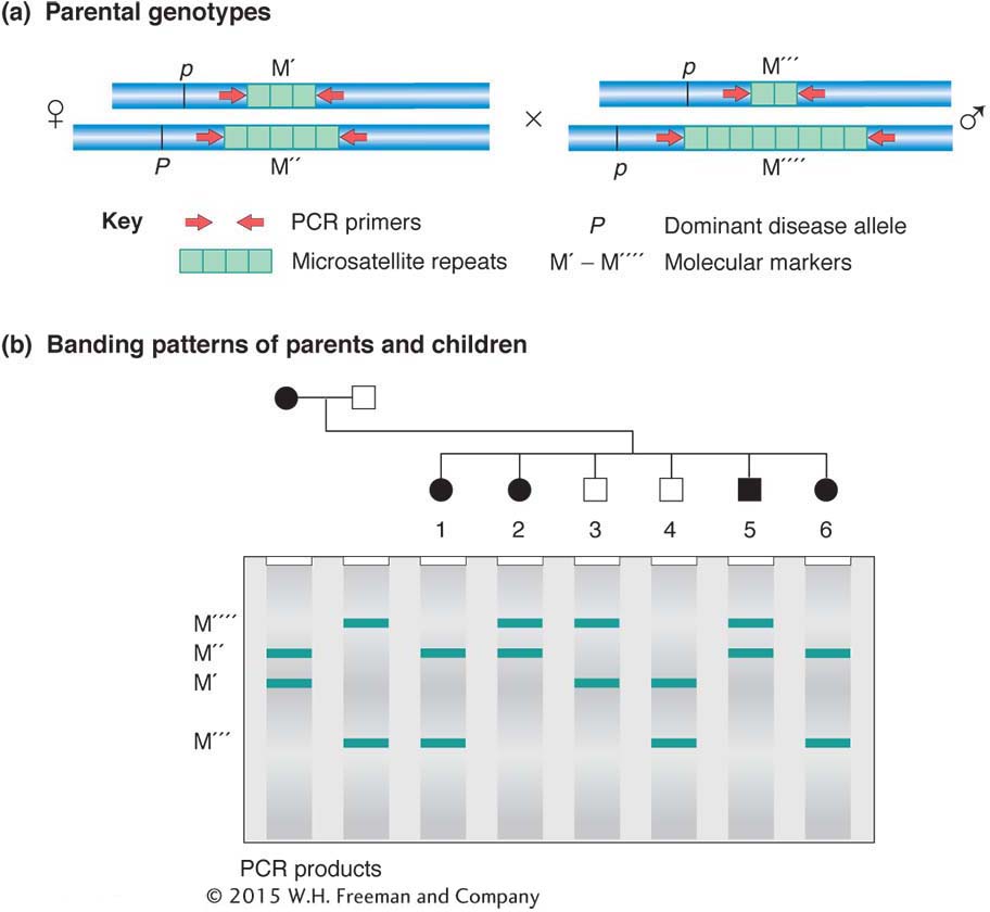
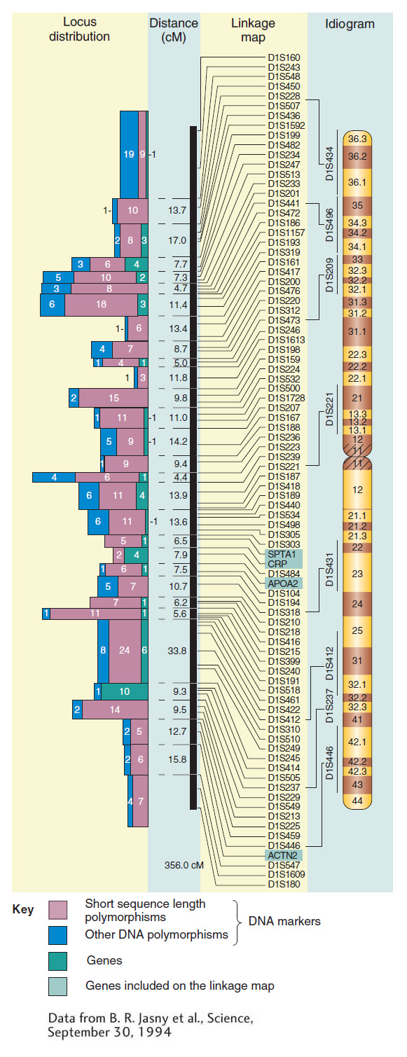
Figure 4-16 contains some real data showing how molecular markers can flesh out a map of a human chromosome. You can see that the number of mapped molecular markers greatly exceeds the number of mapped genes with mutant phenotypes. Note that SNPs, because of their even higher density, cannot be represented on a whole-chromosome map such as that in Figure 4-16, inasmuch as there would be thousands of them. One centimorgan (1 m.u.) of human DNA is a huge segment, estimated as 1 megabase (1 Mb = 1 million base pairs, or 1000 kb). Hence, you can see the need for closely packed molecular markers for a fine-scale analysis that resolves smaller distances. Note that the DNA equivalent of 1 m.u. varies a lot between species; for example, in the malarial parasite Plasmodium falciparium, 1 m.u. = 17 kb.

148