In the discussion of the three-point testcross, some parental (nonrecombinant) chromatids resulted from double crossovers. These crossovers initially could not be counted in the recombinant frequency, skewing the results. This situation leads to the worrisome notion that all map distances based on recombinant frequency might be underestimations of physical distances because undetected multiple crossovers might have occurred, some of whose products would not be recombinant. Several creative mathematical approaches have been designed to get around the multiple-crossover problem. We will look at two methods. First, we examine a method originally worked out by J. B. S. Haldane in the early years of genetics.

The approach worked out by Haldane was to devise a mapping function, a formula that relates an observed recombinant-frequency value to a map distance corrected for multiple crossovers. The approach works by relating RF to the mean number of crossovers, m, that must have taken place in that chromosomal segment per meiosis and then deducing what map distance this m value should have produced.

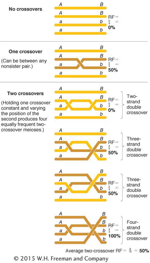
To find the relation of RF to m, we must first think about outcomes of the various crossover possibilities. In any chromosomal region, we might expect meioses with 0, 1, 2, 3, 4, or more crossovers. Surprisingly, the only class that is really crucial is the zero class. To see why, consider the following. It is a curious but nonintuitive fact that any number of crossovers produces a frequency of 50 percent recombinants within those meioses. Figure 4-19 proves this statement for single and double crossovers as examples, but it is true for any number of crossovers. Hence, the true determinant of RF is the relative sizes of the classes with no crossovers (the zero class) compared with the classes with any nonzero number of crossovers.

Now the task is to calculate the size of the zero class. The occurrence of crossovers in a specific chromosomal region is well described by a statistical distribution called the Poisson distribution. The Poisson formula in general describes the distribution of “successes” in samples when the average probability of successes is low. An illustrative example is to dip a child’s net into a pond of fish: most dips will produce no fish, a smaller proportion will produce one fish, an even smaller proportion two, and so on. This analogy can be directly applied to a chromosomal region, which will have 0, 1, 2, and so forth, crossover “successes” in different meioses. The Poisson formula, given here, will tell us the proportion of the classes with different numbers of crossovers:

152

f_i = (e^-mmⁱ)/i!

The terms in the formula have the following meanings:

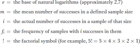
The Poisson distribution tells us that the frequency of the i = 0 class (the key one) is

Because m⁰ and 0! both equal 1, the formula reduces to e^–m.

Now we can write a function that relates RF to m. The frequency of the class with any nonzero number of crossovers will be 1 – e^–m, and, in these meioses, 50 percent (1/2) of the products will be recombinant; so

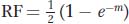
and this formula is the mapping function that we have been seeking.

Let’s look at an example in which RF is converted into a map distance corrected for multiple crossovers. Assume that, in one testcross, we obtain an RF value of 275 percent (0.275). Plugging this into the function allows us to solve for m:

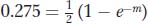
so

By using a calculator to find the natural logarithm (ln) of 0.45, we can deduce that m = 0.8. That is, on average, there are 0.8 crossovers per meiosis in that chromosomal region.

The final step is to convert this measure of crossover frequency to give a “corrected” map distance. All that we have to do to convert into corrected map units is to multiply the calculated average crossover frequency by 50 because, on average, a crossover produces a recombinant frequency of 50 percent. Hence, in the preceding numerical example, the m value of 0.8 can be converted into a corrected recombinant fraction of 0.8 × 50 = 40 corrected m.u. We see that, indeed, this value is substantially larger than the 27.5 m.u. that we would have deduced from the observed RF.

Note that the mapping function neatly explains why the maximum RF value for linked genes is 50 percent. As m gets very large, e^-m tends to zero and the RF tends to 1/2, or 50 percent.

For fungi and other tetrad-producing organisms, there is another way of compensating for multiple crossovers—specifically, double crossovers (the most common type expected). In tetrad analysis of “dihybrids” generally, only three types of tetrads are possible, when classified on the basis of the presence of parental and recombinant genotypes in the products. The classification of tetrads is based on whether there are two genotypes present (ditype) or four (tetratype). Within ditypes there are two classes: parental (showing two parental genotypes) and nonparental (showing two nonparental genotypes). From a cross AB × ab, they are

153

The recombinant genotypes are shown in red. If the genes are linked, a simple approach to mapping their distance apart might be to use the following formula:

because this formula gives the percentage of all recombinants. However, in the 1960s, David Perkins developed a formula that compensates for the effects of double crossovers. The Perkins formula thus provides a more accurate estimate of map distance:

corrected map distance = 50(T + 6 NPD)

We will not go through the derivation of this formula other than to say that it is based on the totals of the PD, T, and NPD classes expected from meioses with 0, 1, and 2 crossovers (it assumes that higher numbers are vanishingly rare). Let’s look at an example of its use. In our hypothetical cross of A B × a b, the observed frequencies of the tetrad classes are 0.56 PD, 0.41 T, and 0.03 NPD. By using the Perkins formula, we find the corrected map distance between the a and b loci to be

50[0.41 + (6 × 0.03)] = 50(0.59) = 29.5 m.u.

Let us compare this value with the uncorrected value obtained directly from the RF. By using the same data, we find

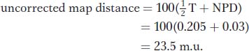
This distance is 6 m.u. less than the estimate that we obtained by using the Perkins formula because we did not correct for double crossovers.

As an aside, what PD, NPD, and T values are expected when dealing with unlinked genes? The sizes of the PD and NPD classes will be equal as a result of independent assortment. The T class can be produced only from a crossover between either of the two loci and their respective centromeres, and, therefore, the size of the T class will depend on the total size of the two regions lying between locus and centromere. However, the formula + NPD should always yield 0.50, reflecting independent assortment.

154