4.7 Using Recombination-Based Maps in Conjunction with Physical Maps
Recombination maps have been the main topic of this chapter. They show the loci of genes for which mutant alleles (and their mutant phenotypes) have been found. The positions of these loci on a map is determined on the basis of the frequency of recombinants at meiosis. The frequency of recombinants is assumed to be proportional to the distance apart of two loci on the chromosome; hence, recombinant frequency becomes the mapping unit. Such recombination-based mapping of genes with known mutant phenotypes has been done for nearly a century. We have seen how sites of molecular heterozygosity (unassociated with mutant phenotypes) also can be incorporated into such recombination maps. Like any heterozygous site, these molecular markers are mapped by recombination and then used to navigate toward a gene of biological interest. We make the perfectly reasonable assumption that a recombination map represents the arrangement of genes on chromosomes, but, as stated earlier, these maps are really hypothetical constructs. In contrast, physical maps are as close to the real genome map as science can get.
The topic of physical maps will be examined more closely in Chapter 14, but we can foreshadow it here. A physical map is simply a map of the actual genomic DNA, a very long DNA nucleotide sequence, showing where genes are, their sequence, how big they are, what is between them, and other landmarks of interest. The units of distance on a physical map are numbers of DNA bases; for convenience, the kilobase is the preferred unit. The complete sequence of a DNA molecule is obtained by sequencing large numbers of small genomic fragments and then assembling them into one whole sequence. The sequence is then scanned by a computer, programmed to look for gene-like segments recognized by characteristic base sequences including known signal sequences for the initiation and termination of transcription. When the computer’s program finds a gene, it compares its sequence with the public database of other sequenced genes for which functions have been discovered in other organisms. In many cases, there is a “hit”; in other words, the sequence closely resembles that of a gene of known function in another species. In such cases, the functions of the two genes also may be similar. The sequence similarity (often close to 100 percent) is explained by the inheritance of the gene from some common ancestor and the general conservation of functional sequences through evolutionary time. Other genes discovered by the computer show no sequence similarity to any gene of known function. Hence, they can be considered “genes in search of a function.” In reality, of course, it is the researcher, not the gene, who searches and who must find the function. Sequencing different individual members of a population also can yield sites of molecular heterozygosity, which, just as they do in recombination maps, act as orientation markers on the physical map.
Because physical maps are now available for most of the main genetic model organisms, is there really any need for recombination maps? Could they be considered outmoded? The answer is that both maps are used in conjunction with each other to “triangulate” in determining gene function, a principle illustrated earlier by the London maps. The general approach is illustrated in Figure 4-20, which shows a physical map and a recombination map of the same region of a genome. Both maps contain genes and molecular markers. In the lower part of Figure 4-20, we see a section of a recombination-based map, with positions of genes for which mutant phenotypes have been found and mapped. Not all the genes in that segment are included. For some of these genes, a function may have been discovered on the basis of biochemical or other studies of mutant strains; genes for proteins A and B are examples. The gene in the middle is a “gene of interest” that a researcher has found to affect the aspect of development being studied. To determine its function, the physical map can be useful. The genes in the physical map that are in the general region of the gene of interest on the recombination map become candidate genes, any one of which could be the gene of interest. Further studies are needed to narrow the choice to one. If that single case is a gene whose function is known for other organisms, then a function for the gene of interest is suggested. In this way, the phenotype mapped on the recombination map can be tied to a function deduced from the physical map. Molecular markers on both maps (not shown in Figure 4-20) can be aligned to help in the zeroing-in process. Hence, we see that both maps contain elements of function: the physical map shows a gene’s possible action at the cellular level, whereas the recombination map contains information related to the effect of the gene at the phenotypic level. At some stage, the two have to be melded to understand the gene’s contribution to the development of the organism.
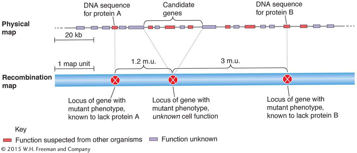
Figure 4-20: Alignment of physical and recombination maps
Figure 4-20: Comparison of relative positions on physical and recombination maps can connect phenotype with an unknown gene function.
There are several other genetic-mapping techniques, some of which we will encounter in Chapters 5, 18, and 19.
KEY CONCEPT
The union of recombination and physical maps can ascribe biochemical function to a gene identified by its mutant phenotype.