5.6 Physical Maps and Linkage Maps compared
Some very detailed chromosomal maps for bacteria have been obtained by combining the mapping techniques of interrupted mating, recombination mapping, transformation, and transduction. Today, new genetic markers are typically mapped first into a segment of about 10 to 15 map minutes by using interrupted mating. Then additional, closely linked markers can be mapped in a more fine-
202
203
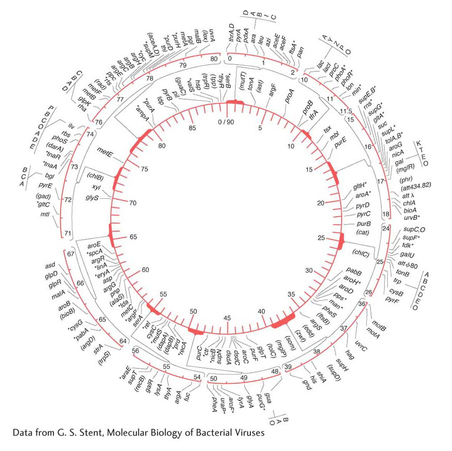
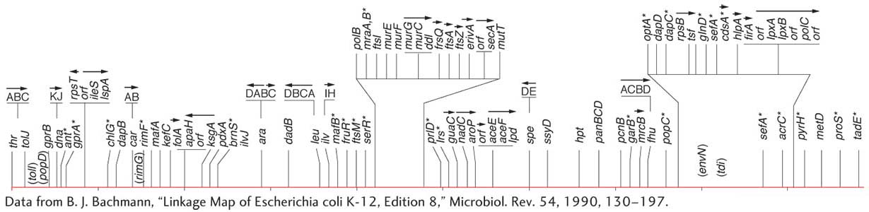
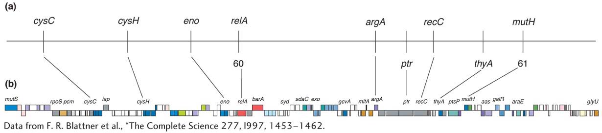
By 1963, the E. coli map (Figure 5-34) already detailed the positions of approximately 100 genes. After 27 years of further refinement, the 1990 map depicted the positions of more than 1400 genes. Figure 5-35 shows a 5-
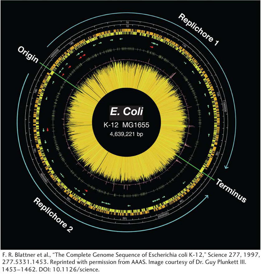
The DNA replication origin and terminus are marked.
The two scales are in DNA base pairs and in minutes.
The orange and yellow histograms show the distribution of genes on the two different DNA strands.
The arrows represent genes for rRNA (red) and tRNA (green).
The central “starburst” is a histogram of each gene with lines of length that reflect predicted level of transcription.
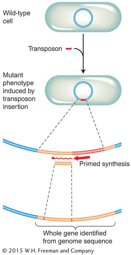
Chapter 4 considered some ways in which the physical map (usually the full genome sequence) can be useful in mapping new mutations. In bacteria, the technique of insertional mutagenesis is another way to zero in rapidly on a mutation’s position on a known physical map. The technique causes mutations through the random insertion of “foreign” DNA fragments. The inserts inactivate any gene in which they land by interrupting the transcriptional unit. Transposons are particularly useful inserts for this purpose in several model organisms, including bacteria. To map a new mutation, the procedure is as follows. The DNA of a transposon carrying a resistance allele or other selectable marker is introduced by transformation into bacterial recipients that have no active transposons. The transposons insert more or less randomly, and any that land in the middle of a gene cause a mutation. A subset of all mutants obtained will have phenotypes relevant to the bacterial process under study, and these phenotypes become the focus of the analysis.
204
The beauty of inserting transposons is that, because their sequence is known, the mutant gene can be located and sequenced. DNA replication primers are created that match the known sequence of the transposon (see Chapter 10). These primers are used to initiate a sequencing analysis that proceeds outward from the transposon into the surrounding gene. The short sequence obtained can then be fed into a computer and compared with the complete genome sequence. From this analysis, the position of the gene and its full sequence are obtained. The function of a homolog of this gene might already have been deduced in other organisms. Hence, you can see that this approach (like that introduced in Chapter 4) is another way of uniting mutant phenotype with map position and potential function. Figure 5-38 summarizes the approach.
As an aside in closing, it is interesting that many of the historical experiments revealing the circularity of bacterial and plasmid genomes coincided with the publication and popularization of J. R. R. Tolkien’s The Lord of the Rings. Consequently, a review of bacterial genetics at that time led off with the following quotation from the trilogy:
One Ring to rule them all, One Ring to find them,
One Ring to bring them all and in the darkness bind them.