The methods of population genetics can be used to analyze any variable or polymorphic locus in the DNA sequences of a population of organisms. Historically, geneticists lacked the molecular tools needed to observe differences in the DNA sequences among individuals directly, and so most population genetic analyses looked at differences in proteins or phenotypes. For example, differences in the protein encoded by the ABO glycosyltransferase gene controlling the ABO blood group in humans can be detected using antibody probes. From these protein differences, investigators can infer differences in the DNA sequence of this gene among individuals. Over the past three decades, new technologies, such as DNA sequencing, DNA microarrays, and PCR (see Chapters 10 and 14), have been developed that allow geneticists to observe differences in the DNA sequences directly. As a result, population genetic analyses are no longer confined to a small set of genes such as ABO but have expanded to include every nucleotide in the genome.

667

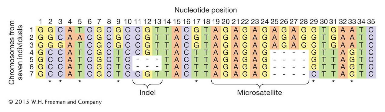
In population genetics, a locus is simply a location in the genome; it can be a single nucleotide site or a stretch of many nucleotides. The simplest form of variation one might observe among individuals at a locus is a difference in the nucleotide present at a single nucleotide site, whether adenine, cytosine, guanine, or thymine. These types of variants are called single nucleotide polymorphisms (SNPs), and they are the most widely studied variants in human population genetics (Figure 18-1; see also Chapter 4). Population genetics also makes extensive use of microsatellite loci (see Chapter 4). These loci have a short sequence motif, 2 to 6 base pairs long, that is repeated multiple times with different alleles having different numbers of repeats. For example, the 2-bp-sequence motif AG at a locus might be tandemly repeated five times in one allele (AGAGAGAGAG) but three times in another (AGAGAG) (see Figure 18-1).

SNPs are the most prevalent types of polymorphism in most genomes. Most SNPs have just two alleles—for example, A and C. SNPs are usually considered common SNPs in a population if the less common allele occurs at a frequency of about 5 percent or greater. SNPs for which the less common allele occurs at a frequency below 5 percent are considered rare SNPs. For humans, there is a common SNP about every 300 to 1000 bp in the genome. Of course, there are a far greater number of rare SNPs.

SNPs occur within genes, including within exons, introns, and regulatory regions. SNPs within protein-coding regions can be classified into one of three groups: synonymous if the different alleles encode the same amino acid, nonsynonymous if the two alleles encode different amino acids, and nonsense if one allele encodes a stop codon and the other an amino acid. Thus, it is sometimes possible to associate a SNP with functional variation in proteins and an associated change in phenotype. SNPs located outside of coding sequences are called noncoding SNPs (ncSNPs). If ncSNPs have no effect on gene function and phenotype, they are called silent. Silent ncSNPs can be very useful in population genetics since they can be used as markers to address questions about population-genetic processes such as gene flow between populations.

668

To study SNP variation in a population, we first need to determine which nucleotide sites in the genome are variable—that is, constitute a SNP. This first step is called SNP discovery. SNPs are often discovered by sequencing the genomes of a small sample of individuals of a species, then comparing these sequences. For example, SNP discovery in humans began by partially sequencing the genomes of a discovery panel of 48 individuals from around the world. Variable nucleotide sites were discovered by comparing the partial genome sequences of these 48 individuals with one another. This initial effort led to the discovery of more than 1 million SNPs.

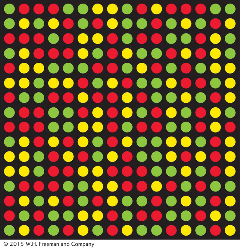
Once SNPs have been discovered, the genotype (allelic composition) of different individuals in the population at each SNP can be determined. DNA microarrays are a widely used technology for this purpose (Figure 18-2). The microarrays used for SNP assays can contain thousands of probes corresponding to known SNPs. Biotechnologists have developed several different methods to detect SNP variants using microarrays. In one method, DNA from an individual is labeled with fluorescent tags and hybridized to the microarray. Each spot (SNP) on the microarray will fluoresce red for one homozygous class, green for the other homozygote, and yellow for a heterozygote (see Figure 18-2). The entire procedure has been enhanced with robotics to allow rapid genotyping, or assignment of genotypes (for example, A/A versus A/C) on a large-scale basis.

Microsatellites are powerful loci for population genetic analysis for several reasons. First, unlike SNPs, which typically have only two alleles per locus and can never have more than four alleles, the number of alleles at a microsatellite is often very large (20 or more). Second, they have a high mutation rate, typically in the range of 10⁻³ to 10⁻⁴ mutations per locus per generation as compared to 10⁻⁸ to 10⁻⁹ mutations per site per generation for SNPs. The high mutation rate means that levels of variation are higher: more alleles per locus and a greater chance that any two individuals will have different genotypes. Third, microsatellites are very abundant in most genomes. Humans have over a million microsatellites.

Microsatellites are found throughout the genomes of most organisms and may be present in exons, introns, regulatory regions, and nonfunctional DNA sequences. Microsatellites with trinucleotide repeats are found in the coding sequences of some genes; these encode strings of a single amino acid. The Huntington disease gene (HD) (see Chapter 16) contains a repeat of CAG, which encodes a string of glutamines. Individuals carrying alleles with more than 30 glutamines are predisposed to develop the disease. In general, however, most microsatellites are located outside of coding sequences, and variation in the number of repeats is not associated with differences in phenotype.

Two main methods are used to discover microsatellite loci in the genome. If a complete genomic sequence is available for an organism, one can simply conduct a search to find them using a computer. For species without genome sequences (most non–model organisms), considerable laboratory work is required to discover microsatellites. Typically, one creates a genomic library, screens the library with a probe for the motif of interest (for example, AG repeats), and determines the DNA sequence of the selected clones to identify the microsatellites and the sequences that flank them. The molecular methods for doing this type of work were discussed in Chapter 10.

669

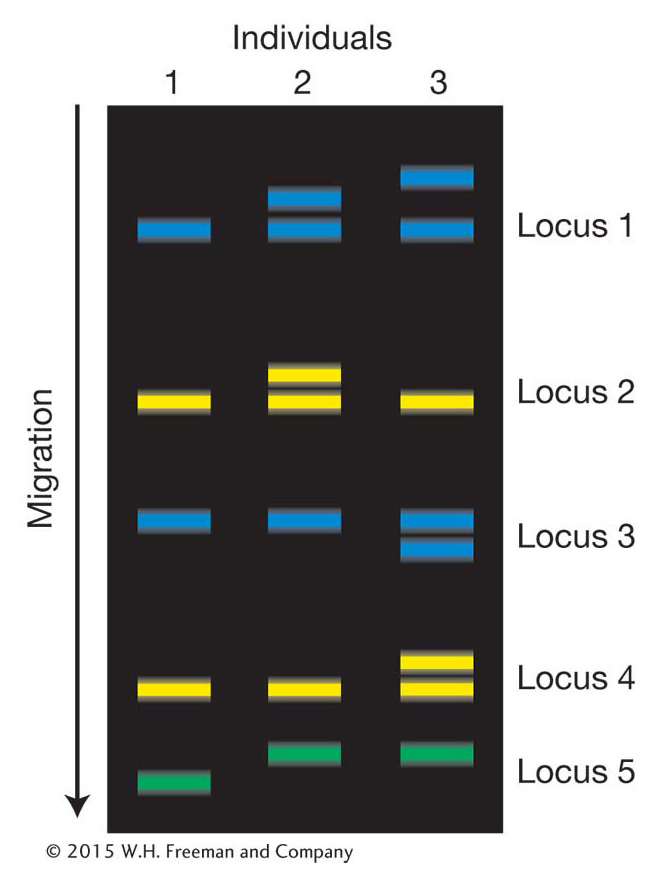
Once a microsatellite and its flanking sequences have been identified, DNA samples from a set of individuals in the population can be analyzed to determine the number of repeats that are present in each individual. To carry out the analysis, oligonucleotide primers are designed that match the flanking sequences for use in PCR. If the primers are labeled with a fluorescent tag, then the sizes of the PCR products can be determined on the same apparatus used to determine the sequence of DNA molecules (Figure 18-3). These sizes reveal the number of repeats in a microsatellite allele. For example, the PCR product of a microsatellite allele containing seven AG repeats will be 8 bp longer than an allele containing three AG repeats. Heterozygous individuals will possess products of two different sizes. Since PCR, the sizing of PCR products, and scoring of the alleles can all be automated, it is possible to determine the genotypes of large samples of individuals for large numbers of microsatellites relatively rapidly.

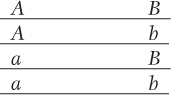
For some questions in population genetics, it is important to consider the genotypes of linked loci as a group rather than individually. Geneticists use the term haplotype to refer to the combination of alleles at multiple loci on the same chromosomal homolog. Two homologous chromosomes that share the same allele at each of the loci under consideration have the same haplotype. If two chromosomes have different genotypes at even one of the loci in question, then they have different haplotypes. If the A locus with alleles A and a is linked to the B locus with alleles B and b, then there are four possible haplotypes for the chromosomal segment on which these two loci are located:

A more complex, but more realistic, example is shown in Figure 18-4. In Figure 18-4a, there are seven chromosome segments but only six haplotypes because chromosome segments 5 and 6 have the same haplotype (E).

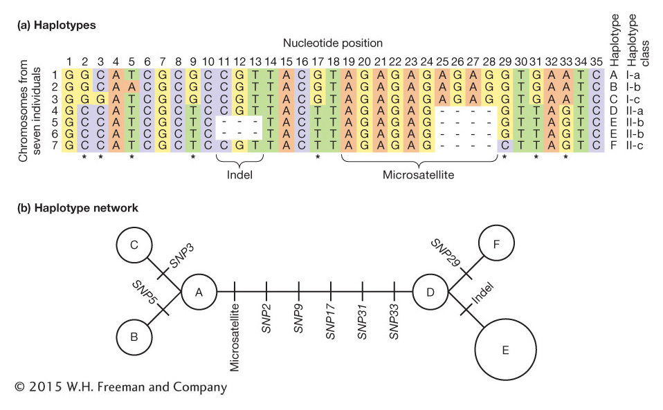
Haplotypes are most often used in population genetics for loci that are physically close. For example, the variable-nucleotide sites in a single gene can be used to define haplotypes for that gene. However, the haplotype concept works for larger regions when there is little or no recombination over the region. It can even be applied to an entire chromosome such as the human Y chromosome. Finally, it is sometimes useful to group haplotypes into classes. As shown in Figure 18-4a, there are two major classes of haplotypes (I and II) that differ at five nucleotide sites plus a microsatellite. However, each class contains several subtypes (I-a, I-b, …). The haplotype network shows the relationships among the haplotypes, placing each mutation on one of the branches (Figure 18-4b).

What insights can we gain from haplotype analysis? Population geneticists studying the human Y chromosome among Asian men discovered one highly prevalent haplotype, termed the “star-cluster” haplotype (Figure 18-5a). Typically, most men have a rare Y chromosome haplotype, but the “star-cluster” haplotype is present in 8 percent of Asian men. Using the known mutation rate, the researchers estimated that this common haplotype arose between 700 and 1300 years ago. (Later in this chapter, we will discuss mutation rates and their use in population genetics.) This haplotype is most common in Mongolia, suggesting that it arose there. The researchers inferred that the “star-cluster” haplotype traces back to one man in Mongolia about 1000 years ago. Remarkably, the present-day distribution of this haplotype follows the geographic boundaries of the Mongolian Empire established by Genghis Khan about 1200 years ago (Figure 18-5b). It appears that contemporary men with this haplotype are all descendants of Genghis Khan (or his male-lineage relatives).

670

Beyond SNP and microsatellites, any variation in the DNA sequence of the chromosomes in a population is amenable to population genetic analysis. Variations that can be analyzed include inversions, translocations, deletions or duplications, and the presence or absence of a transposable element at a particular locus in the genome. Another common form of variation is insertion-deletion polymorphism, or indel for short (see Chapter 16). This type of polymorphism involves the presence or absence of one or more nucleotides at a locus in one allele relative to another. In Figure 18-1, chromosome segments 5 and 6 differ from the other five segments by a 3-bp indel. Unlike microsatellites, indels do not contain repeat motifs such as AGAGAGAG.

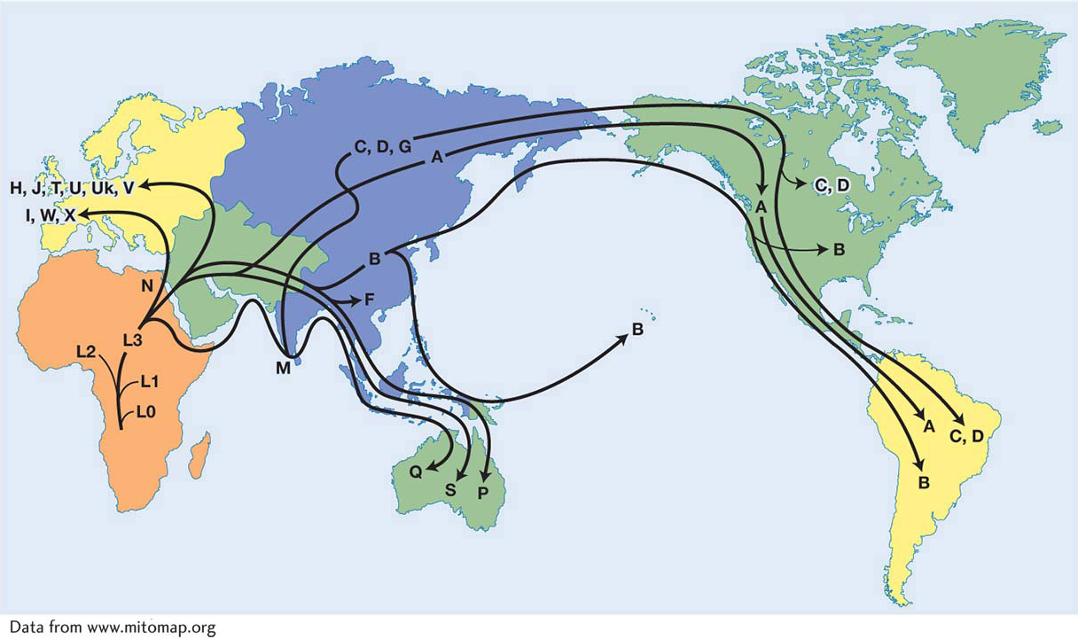
Thus far, our discussion of SNP and microsatellites has focused on the nuclear genome. However, interesting genetic variation can also be found in the mitochondrial (mtDNA) and chloroplast (cpDNA) genomes of eukaryotes. Both SNP and microsatellites are found in these organelle genomes. Since mtDNA and cpDNA are usually maternally inherited, their analysis can be used to follow the history of female lineages. In 1987, a prominent study of the human mitochondrial lineage traced the history of the human mtDNA haplotypes and determined that the mitochondrial genomes of all modern humans trace back to a single woman who lived in Africa about 150,000 years ago (Figure 18-6). She was dubbed the “mitochondrial Eve” in the popular press. This study of mtDNA was the first thorough genetic analysis to suggest that all modern humans came from Africa.

671

A major advance in human population genetics over the past decade was the creation of a genome-wide haplotype map, or HapMap. A consortium of scientists around the world genotyped thousands of people representing the diversity of our species for hundreds of thousands of SNPs and microsatellites. The result is a highly detailed picture of variation in our species. The data are available to the public at several Web sites, including that of the International HapMap Project (www.hapmap.org) and the Human Genome Diversity Project (hgdp.uchicago.edu). In this chapter, we will use these data to present the principles of population genetics. Although first developed for humans, HapMaps have since been developed for several other species, including Drosophila, mouse, Arabidopsis, rice, and maize.

672