Perhaps you have watched someone performing a death-defying stunt and thought that they were at risk of eliminating themselves from the “gene pool.” If so, you were using a concept, the gene pool, that comes straight out of population genetics and has worked its way into popular culture. The gene-pool concept is a basic tool for thinking about genetic variation in populations. We can define the gene pool as the sum total of all alleles in the breeding members of a population at a given time. For example, Figure 18-7 shows a population of 16 frogs, each of which carries two alleles at the autosomal locus A. By simple counting, we can determine that there are five A/A homozygotes, eight A/a heterozygotes, and three a/a homozygotes. The size of the population, usually symbolized by the letter N, is 16, and there is a total of 32 or 2N alleles in this diploid population. With this simple set of numbers, we have described the gene pool with regard to the A locus.

673

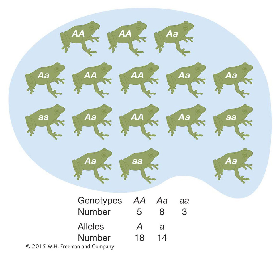
Typically, population geneticists do not care about the absolute counts of the different genotypes in a population but about the genotype frequencies. We can calculate the frequency of the A/A genotype simply by dividing the number of A/A individuals by the total number of individuals in the population (N) to get 0.31. The frequency of A/a heterozygotes is 0.50, and the frequency of a/a homozygotes is 0.19. Since these are frequencies, they sum to 1.0. Frequencies are a more practical measurement than absolute counts because rarely are population geneticists able to study every individual in a population. Rather, population geneticists will draw a random or unbiased sample of individuals from a population and use the sample to infer the genotype frequencies in the entire population.

We can make a simpler description of this frog gene pool if we calculate the allele frequencies rather than the genotype frequencies (Box 18-1). In Figure 18-7, 18 of the 32 alleles are A, so the frequency of A is 18/32 = 0.56. The frequency of the A allele is typically symbolized by the letter p, and in this case p = 0.56. The frequency of the a allele is symbolized by the letter q, and in this case q = 14/32 = 0.44. Again, since these are frequencies, they sum to 1.0: p + q = 0.56 + 0.44 = 1.0. We now have a description of our frog gene pool using only two numbers, p and q.

As mentioned above, an important goal of population genetics is to understand the transmission of alleles from one generation to the next in natural populations. In this section, we will begin to look at how this works. We will see how we can use the allele frequencies in the gene pool to make predictions about the genotype frequencies in the next generation.

The frequency of an allele in the gene pool is equal to the probability that the allele will be chosen when randomly picking an allele from the gene pool to form an egg or a sperm. Knowing this, we can calculate the probability that a frog in the next generation will be an A/A homozygote. If we reach into the frog gene pool (see Figure 18-7) and pick the first allele, the probability that it will be an A is p = 0.56, and similarly the probability that the second allele we pick is also an A is p = 0.56. The product of these two probabilities, or p² = 0.3136, is the probability that a frog in the next generation will be A/A. The probability that a frog in the next generation will be a/a is q² = 0.44 × 0.44 = 0.1936. There are two ways to make a heterozygote. We might first pick an A with probability p and then pick an a with probability q, or we might pick the a first and the A second. Thus, the probability that a frog in the next generation will be heterozygous A/a is pq + qp = 2pq = 0.4928. Overall, the frequencies (f) of the genotypes are

674

Finally, as expected, the sum of the probability of being A/A plus the probability of being A/a plus the probability of being a/a is 1.0:

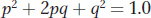
This simple equation is the Hardy-Weinberg law, and it is part of the foundation for the theory of population genetics.

The process of reaching into the gene pool to pick an allele is called sampling the gene pool. Since any individual that contributes to the gene can produce many eggs or sperm that carry exactly the same copy of an allele, it is possible to pick a particular copy and then reach back into the gene pool and pick exactly the same copy again. There is also an element of chance involved when sampling the gene pool. Just by chance, some copies may be picked more than once and other copies may not be picked at all. Later in the chapter, we will look at how these properties of sampling the gene pool can lead to changes in the gene pool over time.

We used the Hardy–Weinberg law to calculate genotype frequencies in the next generation from the allele frequencies in the current generation. We can also use the Hardy–Weinberg law to calculate allele frequencies from the genotype frequencies within a single generation. For example, some forms of albinism in humans are due to recessive alleles at the OCA2 locus. In Africa, a form of albinism called brown oculocutaneous albinism results from a recessive allele of OCA2 (Figure 18-8). Individuals with this condition are present at frequencies as high as 1 in 1100 among some ethnic groups in Africa. We can use the Hardy–Weinberg law to calculate the allele frequencies:

so

and

Using the allele frequencies, we can also calculate the frequency of heterozygotes in the population as

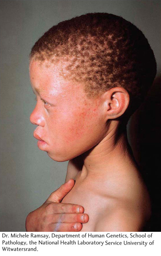
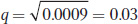
The latter number predicts that about 6 percent of this population are heterozygotes, or carriers of the recessive allele at OCA2.

When we use the Hardy–Weinberg law to calculate allele or genotype frequencies, we make some critical assumptions.

675

We have seen how we can use the Hardy–Weinberg law and the gene frequencies in the current generation (t₀) to calculate genotype frequencies in the next generation (t₁) by randomly sampling the gene pool for the production of eggs and sperm. Similarly, the predicted genotype frequencies for generation t₁ can be used in turn to calculate gene frequencies for the next generation (t₂). The gene frequencies in generation t₂ will remain the same as generation t₁. Under the Hardy–Weinberg law, neither gene nor genotype frequencies change from one generation to the next when an infinitely large population is randomly sampled for the formation of eggs and sperm. Thus, an important lesson from the Hardy–Weinberg law is that, in large populations, genetic variation is neither created nor destroyed by the process of transmitting genes from one generation to the next. Populations that adhere to this principle are said to be at Hardy-Weinberg equilibrium.

Here are a few more points about the Hardy–Weinberg law.

1. For any allele that exists at a very low frequency, homozygous individuals will only very rarely be found. If allele a has a frequency of 1 in a thousand (q = 0.001), then only 1 in a million (q²) individuals will be homozygous for that allele. As a consequence, recessive alleles for genetic disorders can occur in the heterozygous state in many more individuals than there are individuals that actually express the genetic disorder in question.

2. The Hardy–Weinberg law still applies where there are more than two alleles per locus. If there are n alleles, A₁, A₂, … A_n with frequencies p₁, p₂, … p_n, then the sum of all the individual frequencies equals 1.0. The frequencies of each of the homozygous genotypes are simply the square of the frequencies of the alleles, and the frequencies of the different heterozygous classes are two times the product of the frequencies of the first and second allele. Table 18-1 gives an example with p₁ = 0.5, p₂ = 0.3, and p₃ = 0.2.

676

3. Hardy–Weinberg logic applies to X-linked loci as well. Males are hemizygous for X-linked genes, meaning that a male has a single copy of these genes. Thus, for X-linked genes in males, the genotype frequencies are equal to the allele frequencies. For females, genotype frequencies for X-linked genes follow normal Hardy–Weinberg expectations.

Male pattern baldness is an X-linked trait (Figure 18-9). AR (for androgen receptor) is an X-linked gene involved in male development. There is an AR haplotype called Eur-H1 that is strongly associated with pattern baldness. Male pattern baldness is common in Europe, where the Eur-H1 haplotype occurs at a frequency of 0.71, meaning that 71 percent of European men carry it. Using the Hardy–Weinberg law, we can calculate that 50 percent of European women are Eur-H1 homozygotes and 41 percent are heterozygous. The inheritance of baldness is complex and is affected by multiple genes, and so not all men who have Eur-H1 go bald.

4. One can test whether the observed genotype frequencies at a locus fit Hardy–Weinberg predictions using the χ² test (see Chapter 3). An example is provided by the human leukocyte antigen gene, HLA-DQA1, of the major histocompatibility complex (MHC). MHC is a cluster of genes on chromosome 6 that play roles in the immune system. Table 18-2 has genotype frequencies for a SNP (rs9272426) in the HLA-DQA1 for 84 residents of Tuscany, Italy. This SNP has alleles A and G. From the genotype frequencies in Table 18-2, we can calculate the allele frequencies: f (A) = p = 0.53 and f(G) = q = 0.47. Next, we can calculate expected genotype frequencies under the Hardy–Weinberg law: p² = 0.281, 2pq = 0.498, and q² = 0.221. Multiplying the expected genotype frequencies times the sample size (N = 84) gives us the expected number of individuals for each genotype. Now we can calculate the χ² statistic to be 8.29. Using Table 3-1, we see that the probability under the null hypothesis that the observed data fit Hardy–Weinberg predictions is P < 0.005 with df = 1. [We have only one degree of freedom because we have three genotypic categories and we used two numbers from the data (N and p) to calculate the expected values (3 − 2 leaves 1 degree of freedom). We did not need to use q since q = p − 1.] This analysis makes us strongly suspect that Tuscans do not conform to Hardy–Weinberg expectations with regard to HLA-DQA1. We will look further at the population genetics of MHC in Section 18.3 on mating systems and Section 18.5 on natural selection.

The Hardy–Weinberg law is part of the foundation of population genetics. It applies to an idealized population that is infinite in size and in which mating is random. It also assumes that all genotypes are equally fit—that is, that they are all equally viable and have the same success at reproduction. Real populations deviate from this idealized one. In the rest of the chapter, we will examine how factors such as nonrandom mating, finite population size, and the unequal fitness of different genotypes cause deviations from Hardy–Weinberg expectations. We will also see how the Hardy–Weinberg law can be modified to compensate for these factors.

677