To study the inheritance of quantitative traits, we need some basic statistical tools. In this section, we will introduce the mean (or average), which can be used to describe differences between groups, and the variance, which can be used to quantify the amount of variation that exists within a group. We will also discuss the normal distribution, which is central to understanding quantitative variation in populations. But before discussing the statistical tools, let’s define the different types of complex trait variation that can occur in a population.

A continuous trait is one that can take on a potentially infinite number of states over a continuous range. Height in humans is a good example. People can range from about 140 cm to 230 cm in height. If we measured height precisely, then the number of possible heights is infinite. For example, a person might be 170 cm tall or 170.2 or 170.0002 cm. Continuous traits typically have complex inheritance involving multiple genes plus environmental factors.

For some traits, the individuals in a population can be sorted into discrete groups or categories. Such traits are known as categorical traits. Examples include purple versus white flowers or tall versus short stems for Mendel’s pea plants, as seen in Chapter 2. Categorical traits often exhibit simple inheritance such that the progeny of crosses segregate into standard Mendelian ratios such as 3:1 for a single gene or 15:1 for two genes. The inheritance is simple because only one or two genes are involved and the environment has little or no effect on the phenotype.

Some categorical traits do not show simple inheritance. These include many disease conditions in humans. In medical genetics, individuals can be classified into the categories “affected” or “not affected” by a disease. For example, an individual may or may not have type 2 diabetes. However, type 2 diabetes does not follow simple Mendelian rules or produce Mendelian ratios in pedigrees. Rather, there are multiple genetic and environmental factors that place someone at risk of developing this disease. Individuals who have a certain number of risk factors will exceed a threshold and develop the disease. Type 2 diabetes is a form of a categorical trait called a threshold trait. Type 2 diabetes has complex inheritance.

718

Another type of trait is a meristic trait, or counting trait, which takes on a range of discrete values. An example would be clutch size in birds. A bird can lay 1, 2, 3, or more eggs, but it cannot lay 2.49 eggs. Meristic traits are quantitative, but they are restricted to certain discrete values. They do not take on a continuous range of values. Meristic traits usually have complex inheritance.

Quantitative geneticists seek to understand the inheritance of traits that show complex inheritance resulting from a mix of genetic and environmental factors. They may investigate traits that are categorical, meristic, or continuous. The emphasis is on the type of inheritance—complex. For this reason, the term complex trait is often preferred to continuous or quantitative trait because it includes all the types of traits with which quantitative genetics is concerned. Any biological phenomenon for which variation exists may show complex inheritance and can be studied as a complex trait. Thus, size and shape of structures, enzyme kinetics, mRNA levels, circadian rhythms, and bird songs can all be treated as complex traits.

When quantitative geneticists study the inheritance of a trait, they work with a particular group of individuals, or population. For example, we might be interested in the inheritance of height for the population of adult men in Shanghai, China. Here, we are using “population” to denote a group that shares certain features in common such as age, sex, ethnicity, or geographic origin. Since there are more than 5 million adult men in Shanghai, determining each of their heights would be a herculean task. Therefore, quantitative geneticists typically study just a subset or sample of the full population. The sample should be randomly chosen such that each of the 5 million men has an equal chance of being included in the sample. If the sample meets this criterion, then we can use measurements made on the sample to make inferences about the entire population.

Using the example of height for men from Shanghai, we can describe the population using the mean or average value for the trait. We select a random sample of 100 men from the population and measure their heights. Some of the men might be 166 cm tall, others 172 cm tall, and so forth. To calculate the mean, we simply sum all the individual measurements and divide the sum by the size of the sample (n), which in this case is 100. For the data in Table 19-1, the result would be 170 cm, or 5 feet, 7 inches. Since we have a random sample, we can infer that the average height in the entire population is 170 cm.

Height is a random variable which means it can take on different values, and when we select someone at random from the population, the value we observe is governed by an element of chance. Random variables are usually represented by the letter X in statistics. We have measurements for X₁, X₂, X₃, … X₁₀₀ for the n = 100 men in the sample. Symbolically, we can express the mean as

where represents the sample mean. The uppercase Greek letter sigma (Σ) is the summation sign, indicating that we add all n observed values of X for i = 1, 2, through n. (Often, the n above Σ and the i = 1 below Σ are omitted to simplify the appearance of equations.)

There is a distinction made between the mean of a sample ( ) and the true mean of the population. To learn the true mean for the height of men in Shanghai, we would need to determine the height of each and every man. The true mean is symbolized by the Greek letter μ, so that we have different symbols for the sample and population means.

719

Here is another way to calculate the mean, which is often quite useful. We can add the products of each class of values of X in the data set times the frequency of that class in the data set. This operation is symbolized as

where f_i is the frequency of the ith class of observations, X_i is the value of the ith class, and there are a total of k classes. For the data in Table 19-1, one man of the 100 (f = 0.01) is 156 cm tall, two men (f = 0.02) are 157 cm tall, and so forth, so we can calculate the sample mean as

The mean is useful for both describing populations and comparing differences between populations. For example, men in urban areas of China are on average 170 cm tall, while men in rural areas of China are 166 cm tall. These values were calculated using samples drawn from each region. One question that a quantitative geneticist might ask about the observed difference in height between rural and urban Chinese men is the following: Is the difference due to genetic factors, or is it due to differences in nutrition, health care, or other environmental factors? Later in the chapter, we’ll see how quantitative geneticists tease apart genetic versus environmental contributions to a trait.

Lastly, here is another helpful notation from statistics that can be used to define the mean. The mean of a random variable, X, is the expectation or expected value of that random variable. The expected value is the average of all the values we would observe if we measured X many times. The expectation is symbolized by E, and we write E(X) to signify “the expected value of X.” Symbolically, we write

We will use the notation of expectation in several places in this chapter.

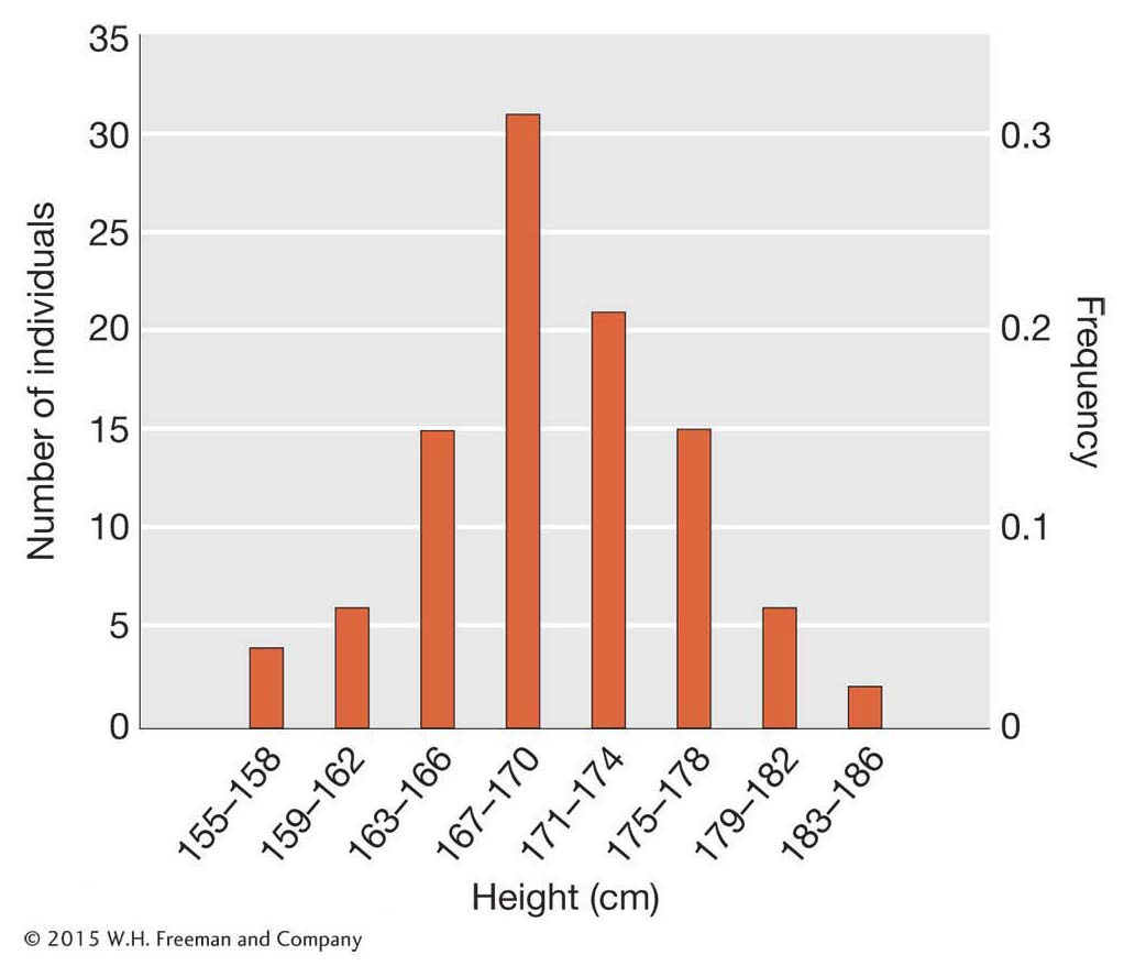
Besides the mean, we also need a measure of how much variation exists in populations. We can create a visual representation of the variation by plotting the count or frequency of each height class. Figure 19-1 shows such a plot for our simulated height data for 100 men from Shanghai. The x-axis shows different height classes, and the y-axis shows the count or frequency of each class. In this figure, the men were binned into 4-cm groups, for example, between 155 and 158 cm. This type of graph is called a frequency histogram. If the values are clustered tightly around the mean, then there is less variation, and if the values are spread out along the x-axis, there is greater variation.

We can quantify the amount of variation in a population using a statistical measure called the variance. The variance measures the extent to which individuals in the population deviate from the population mean. If all 100 men in our sample had heights very close to the mean, then the variance would be small. If their heights deviated greatly from the mean, the variance would be large.

720

Since the variance is a measure of deviation from the mean, let’s define deviation mathematically. Knowing the mean value for the random variable X, we can calculate the deviation of each individual from the mean by subtracting from the individual observations. We will represent the deviations by a lower case x:

Some individuals will have X values above the mean, and they will have a positive deviation. Others will have X values below the mean, and they will have a negative deviation. For the population overall, the expected value of x is 0, or E(x) = 0.

To measure the amount of variation for X in the population, we use the variance, which is the mean of the squared deviations. First, we calculate the sum of the squared deviations (or sum of squares for short) as

Since deviations with negative values form positive squares, both negative and positive deviations will contribute positively to the sum of squares. The variance is the mean of the squared deviations (or the sum of squares divided by n). Symbolically, we express the population variance as

where V_X denotes the variance of X. The population variance is sometimes symbolized using the lowercase Greek letter sigma squared (σ²). In statistics, there is also a distinction made between the population variance (σ²) and the sample variance (s²). The latter is calculated by dividing the sums of squares by n − 1 rather than n to correct a bias caused by small sample size. For simplicity, we will use the population variance and the formula above throughout this chapter.

There are several points to understand about the variance. First, the variance provides a measure of dispersion about the mean. When the variance is high, the individual values are spread farther apart from the mean; when it is low, then the individual values cluster closer to the mean. Second, the variance is measured in squared units such that if we measure human height in centimeters, then the variance would be in centimeters². Third, the variance can range from 0.0 to infinity. Fourth, the variance is equal to the expected value of the squared deviation (x²) or E(x²).

The variance of quantitative traits is measured in squared units. These squared units have desirable mathematical properties as we will see below; however, they do not make intuitive sense. If we measure weight in kilograms, then the variance would be in kilograms², which has no clear meaning. Therefore, another statistic used to quantify the extent of deviation from the mean in a population is the standard deviation (σ), which is the square root of the variance:

The standard deviation is expressed in the same units as the trait itself, so its meaning is more intuitive. We will use the standard deviation in the description of traits below.

721

Even if you have never taken a statistics course, you likely have heard of the normal distribution, also known as the “bell curve” in popular culture. The normal distribution is remarkably useful in biology in general and quantitative genetics in particular because the frequency distribution for many biological traits approximates a normal curve. For this reason, geneticists can take advantage of several features of the normal distribution to describe quantitative traits and dissect the underlying genetics.

The normal distribution is a continuous frequency distribution similar to the frequency histogram shown in Figure 19-1. The normal distribution applies to continuous traits. As mentioned above, continuous traits can take on an infinite number of values. A person might be 170 cm tall or 170.2 or 170.002 and so forth. For such traits, the expected frequency of different trait values is better represented by a curve than by a frequency histogram. For the normal distribution, the shape of the curve is determined by two factors—the mean and the standard deviation.

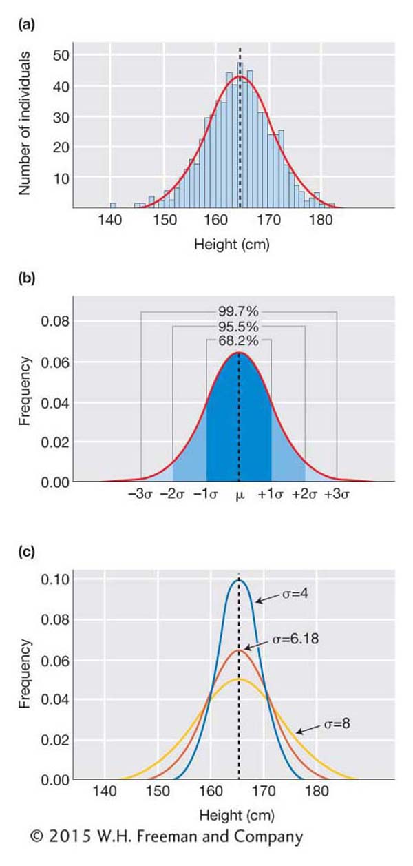
Here is an example using height data for 660 women from the United States collected by the Centers for Disease Control and Prevention. The frequency histogram shows the classic “bell curve” shape with the peak near the mean value of 164.4 cm and the off-mean values distributed symmetrically around the mean (Figure 19-2a). We can fit a normal curve to this distribution using just two pieces of information—the mean and the standard deviation. The shape of the curve is defined by an equation called the normal probability density function, into which the mean and the standard deviation are plugged. The normal distribution allows us to predict the percentage of the observations that will fall within a certain distance from the mean (Figure 19-2b). If we measure distance along the x-axis in standard deviations, then 68 percent of the observations are expected to fall within 1 standard deviation (σ) of the mean and 95.5 percent within 2 standard deviations. For the height data for U.S. women, 71 percent (449 women) fall within 1 standard deviation of the mean and 96 percent (633 women) within 2 standard deviations. These values are very close to the predictions of 68.2 percent and 95.5 percent based on the normal curve.

If we know just the mean and the standard deviation for a trait, we can predict the shape of the distribution of the trait in the population, and we can predict how likely we are to observe certain values when sampling the population. For example, if the mean height for U.S. women is 164.4 cm (5 feet, 5 inches) and the standard deviation is 6.18 cm, we can predict that only 2 percent of women will be more than 177 cm tall, or five feet, 10 inches. As shown in Figure 19-2c, if the standard deviation is greater (for example, 8), then the curve would be flatter and a greater percentage would fall above 177 cm. However, it would still be true that only 2 percent would be more than 2σ above the mean, or 180.4 cm [(164.4 + (2 × 8)].

722