19.3 Broad-Sense Heritability: Nature Versus Nurture
A key question in genetics is, How much of the variation in a population is due to genetic factors and how much to environmental factors? In the popular press, this question is often phrased in terms of nature versus nurture—
Quantitative geneticists have developed the statistical tools needed to estimate, with reasonable precision, the extent to which variation in complex traits is due to genes versus the environment. Below, we will describe these tools. At the end of this section, we will discuss the assumptions underlying these estimates and the limits to their utility.
Let’s begin by defining broad-

728
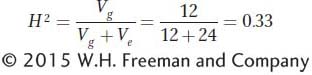
The H is squared because it is the ratio of two variances, which are measured in squared units. H2 can vary from 0 to 1.0. When all of the variation in a population is due to environmental sources and there is no genetic variation, then H2 is 0. When all of the variation in a population is due to genetic sources, then Vg equals VX and H2 is 1.0. H2 is called “broad sense” because it encompasses several different ways by which genes contribute to variation. For example, some of the variation will be due to the contributions of individual genes. Additional genetic variation can be contributed by the way genes work together, the interactions between genes, or epistasis.
In Section 19.2, we showed how we can calculate the genetic and environmental variances when we have inbred lines or clones. For the imaginary example of days to pollen shed for maize inbred lines in Table 19-2 (experiment I), we saw that Vg is 12.0 and VX is 14.67. Using these values, the heritability of the trait is 12.0/14.67 = 0.82, or 82 percent. This estimate of H2 tells us that genes contribute most of the variation and environmental factors contribute a more modest share of the variation. Thus, we might conclude that days to pollen shed is a highly heritable trait in maize.
Let’s look at the data for experiment II in Table 19-2. The genotypes are exactly the same as in experiment I; these are the genotypes of the inbred lines A through J. In this case, however, the lines are reared in more extreme environments. If we calculate the variance for the means of the inbred line in experiment II, Vg will be 12.0 days2 as in experiment I. Since the genotypes are the same in both experiments, the genetic variance is the same. If we calculate the variance for the means of the different environments (Ve) in experiment II, we will obtain 24.0 days2, which is much larger than the value for Ve in experiment I (2.67). Since the environments are more extreme, the environmental variance is larger. Finally, if we calculate H2 for experiment II, we obtain
The estimate of H2 for experiment II is on the small side—
The contrast between the estimates of the heritability for the same set of maize inbred lines reared in different environments highlights the point that heritability is the proportion of the phenotypic variance (VX) due to genetics. Since VX = Vg + Ve, as Ve increases, then Vg will represent a smaller part of VX and H2 will go down. Similarly, if the environmental variance is kept to a minimum, then Vg will represent a larger part of VX and H2 will go up. H2 is a moving target, and results from one study may not apply to another.
Measuring heritability in humans using twin studies

How can we measure heritability in humans? Although we don’t have inbred lines for humans, we do have genetically identical individuals—
The equation for estimating H2 in studies of identical twins who are reared apart is relatively simple. It makes use of the statistical measure called the covariance, which was introduced in Box 19-2. As explained in Box 19-3, the covariance between identical twins who are reared apart is equal to the genetic variance (Vg). Thus, we can estimate H2 in humans by using this covariance as the numerator and the trait variance (Vx) as the denominator:

729
Here’s how it’s done. For each set of twins, let’s designate the trait value for one twin as X′ and the other as X″. If we have n sets of twins, then the trait values for the n sets could be designated  .
.
Suppose we had IQ measurements for five sets of twins as follows:
|
Twin |
||
|---|---|---|
|
X′ |
X″ |
|
|
1 |
100 |
110 |
|
2 |
125 |
118 |
|
3 |
97 |
90 |
|
4 |
92 |
104 |
|
5 |
86 |
89 |
730
Using these data and the formula for the covariance from Box 19-2, we calculate that COVX′,X″ is 119.2 points2. Using the formula for trait variance, we would calculate that the value of VX is 154.3 points2. Thus, we obtain

The points2 in the numerator and denominator cancel out, and we are left with a unitless measure that is the proportion of the total variance that is due to genetics.
Box 19-3 provides some additional details about estimating H2 from twin data, including the derivation of the formula we just used. It also discusses the relationship between the ratio COVX′,X″/VX and the correlation coefficient. Quantitative geneticists have developed several means for estimating heritability using the correlation among relatives. Identical twins share 100 percent of their genes, while brothers, sisters, and dizygotic twins share 50 percent of their genes. The strength of the correlation between different types of relatives can be scaled for the proportion of their genes that they share and the results used to estimate the genetic and environmental contributions to trait variation.
Estimating Heritability from Human Twin Studies
If we had many sets of identical twins who were reared apart, how could we use them to measure H2? Let’s arbitrarily represent the trait value for one member of each pair of twins as X′ and the trait value for the other as X″. We have many (n) sets of twins: 
 . We can express the phenotypic deviations for one set of twins as the sum of their genetic and environmental deviations,

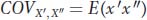
using x′ as the deviation for one twin and x″ for the other twin. Notice that g is the same because the twins are genetically identical, but e′ and e″ are different because the twins were reared in separate households. Next, we develop an expression for the covariance between the twins. In Box 19-2, we saw that the covariance is the average or expected value of the cross products E(xy). Using our notation for twins, x′ and x″, in place of x and y, we get
We can substitute (g + e′) for x′ and (g + e″) for x″, giving us
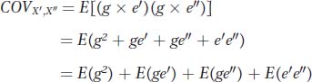
Let’s consider the last three terms of this expression. Under our model, the twins are assigned randomly to households, and thus there should be no correlation between the environments to which the X′ and X″ twin of each pair are assigned. Accordingly, the covariance between the environments [E(e′e″)] will be 0.0. Similarly, because the assignment of twins to households is random, we expect no correlation between the genetic deviation of twins (g) and the household to which they are assigned, so E(ge′) and E(ge″) will be 0.0. Therefore, the equation for the covariance among twins reduces to
In other words, the covariance among identical twins reared apart is equal to the genetic variance. If we have a large set of identical twins who were reared apart, we can use the covariance between the twins to estimate the amount of genetic variation for a trait in the general population. If we divide this covariance by the phenotypic variance, then we have an estimate of H2:

This equation is essentially the correlation coefficient between the twins. The variance for the twin of each set designated X′ and that for the twin designated X″ are expected to be the same over a large sample. Thus, we can rewrite the denominator of the equation as follows:

and we will see that H2 is equivalent to the correlation between twins.
Over the last 100 years, there have been extensive genetic studies of twins and other sets of relatives. A great deal has been learned about heritable variation in humans from these studies. Table 19-4 lists some results from twin studies. It may or may not be surprising to you, but there is a genetic contribution to the variance for many different traits, including physique, physiology, personality attributes, psychiatric disorders, and even our social attitudes and political beliefs. We readily observe that traits such as hair and eye color run in families, and we know these traits are the manifestation of genetically controlled biochemical, developmental processes. In this context, it is not so surprising that other aspects of who we are as people also have a genetic influence.
|
Trait |
H2 |
|---|---|
|
Physical attributes |
|
|
Height |
0.88 |
|
Chest circumference |
0.61 |
|
Waist circumference |
0.25 |
|
Fingerprint ridge count |
0.97 |
|
Systolic blood pressure |
0.64 |
|
Heart rate |
0.49 |
|
Mental attributes |
|
|
IQ |
0.69 |
|
Speed of spatial processing |
0.36 |
|
Speed of information acquisition |
0.20 |
|
Speed of information processing |
0.56 |
|
Personality attributes |
|
|
Extraversion |
0.54 |
|
Conscientiousness |
0.49 |
|
Neuroticism |
0.48 |
|
Positive emotionality |
0.50 |
|
Antisocial behavior in adults |
0.41 |
|
Psychiatric disorders |
|
|
Autism |
0.90 |
|
Schizophrenia |
0.80 |
|
Major depression |
0.37 |
|
Anxiety disorder |
0.30 |
|
Alcoholism |
0.50- |
|
Beliefs and political attitudes |
|
|
Religiosity among adults |
0.30– |
|
Conservatism among adults |
0.45– |
|
Views on school prayer |
0.41 |
|
Views on pacifism |
0.38 |
|
Sources: J. R. Alford et al., American Political Science Review 99, 2005, 1– |
|
Twin studies and the estimates of heritability that they provide can easily be over-
731
Finally, heritability is not useful for interpreting differences between groups. Table 19-4 shows that the heritability for height in humans can be very high: 0.88. However, this high value for heritability does not tell us anything about whether groups with different heights differ because of genetics or the environment. For example, men in the Netherlands today average 184 cm in height, while around 1800, men in the Netherlands were about 168 cm tall on average, a 16-