The genes that control variation in quantitative (or complex) traits are known as quantitative trait loci, or QTL for short. As we will see below, QTL are genes just like any others that you have learned about in this book. They may encode metabolic enzymes, cell-surface proteins, DNA-repair enzymes, transcription factors, or any of many other classes of genes. What is of interest here is that QTL have allelic variants that typically make relatively small, quantitative contributions to the phenotype.

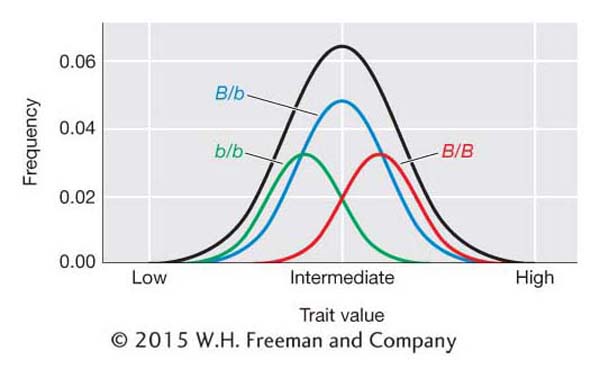
We can visualize the contributions of the alleles at a QTL to the trait value by looking at the frequency distributions associated with each genotype at a QTL as shown in Figure 19-11. The QTL locus is B and the genotypic classes are B/B, B/b, and b/b. The B/B individuals tend to have higher trait values, B/b intermediate values, and b/b small values. However, their distributions overlap, and we cannot determine genotype simply by looking at an individual’s phenotype as we can for genes that segregate in Mendelian ratios. In Figure 19-11, an individual with an intermediate trait value could be either B/B, B/b, or b/b.

Because of this property of QTL, we need special tools to determine their location in the genome and characterize their effects on trait variation. In this section, we will review a powerful form of analysis for accomplishing the first of these goals. This form of analysis is called QTL mapping. Over the past two decades, QTL mapping has revolutionized our understanding of the inheritance of quantitative traits. Pioneering work in QTL mapping was performed with crop plants such as tomato and corn. However, it has been broadly applied in model organisms such as mouse, Drosophila, and Arabidopsis. More recently, evolutionary biologists have employed QTL mapping to investigate the inheritance of quantitative traits in natural populations.

743

The fundamental idea behind QTL mapping is that one can identify the location of QTL in the genome using marker loci linked to a QTL. Here is how the method works. Suppose you make a cross between two inbred strains—parent one (P₁) with a high trait value and parent two (P₂) with a low trait value. The F₁ can be backcrossed to P₁ to create a BC₁ population in which the alleles at all the genes in the two parental genomes will segregate. Marker loci such as SNPs or microsatellites can be scored unambiguously as homozygous P₁ or heterozygous for each BC₁ individual. If there is a QTL linked to the marker locus, then the mean trait value for individuals that are homozygous P₁ at the marker locus will be different from the mean trait value for the heterozygous individuals. Based on such evidence, one can infer that a QTL is located near the marker locus. Let’s look in more detail at how this works.

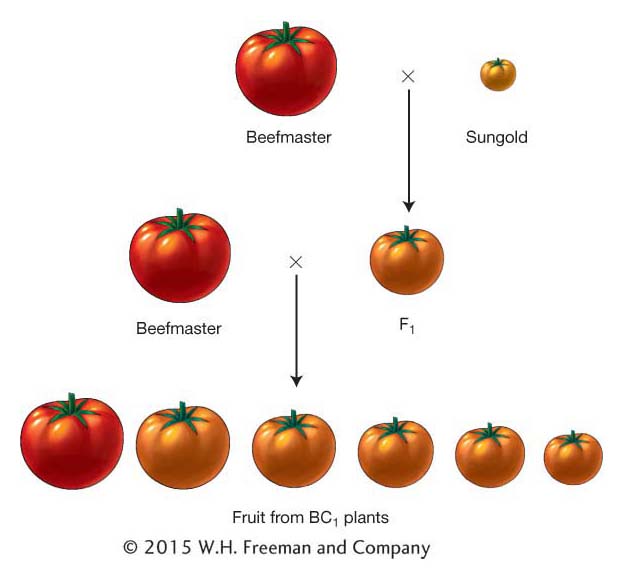
There are a variety of experimental designs that can be used in QTL mapping experiments. We will begin by describing a simple design. Let’s say we have two inbred lines of tomato that differ in fruit weight—Beefmaster with fruits of 230 g in weight and Sungold with fruits of 10 g in weight (Figure 19-12). We cross the two lines to produce an F₁ hybrid and then backcross the F₁ to the Beefmaster line to produce a BC₁ generation. We grow several hundred BC₁ plants to maturity and measure the weight of the fruit on each. We also extract DNA from each of the BC₁ plants. We use these DNA samples to determine the genotype of each plant at a set of marker loci (SNPs or SSRs) that are distributed across all of the chromosomes such that we have a marker locus every 5 to 10 centimorgans.

744

From this process, we would assemble a data set for several hundred plants and 100 or more marker loci distributed around the genome. Table 19-6 shows part of such a data set for just 20 plants and 5 marker loci that are linked on a single chromosome. For each BC₁ plant, we have the weight of its fruit and the genotypes at the marker loci. You’ll notice that trait values for the BC₁ plants are intermediate between the two parents as expected but closer to the Beefmaster value because this is a BC₁ population and Beefmaster was the backcross parent. Also, since this is a backcross population, the genotypes at each marker locus are either homozygous for the Beefmaster allele (B/B) or heterozygous (B/S). In Table 19-6, you can see the positions of crossovers between the marker loci that occurred during meiosis in the F₁ parent of the BC₁ generation. For example, plant BC₁-001 has a recombinant chromosome with a crossover between marker loci M3 and M4.

The overall mean fruit weight for the BC₁ population is 175.7. We can also calculate the mean for the two genotypic classes at each marker locus as shown in Table 19-6. For marker M1, the means for the B/B (176.3) and B/S (175.3) genotypic classes are very close to the overall mean (175.7). This is the expectation if there is no QTL affecting fruit weight near M1. For marker M3, the means for the B/B (180.7) and B/S (169.6) genotypic classes are quite different from the overall mean (175.7) and from each other. This is the expectation if there is a QTL affecting fruit weight near M3. Thus, we have evidence for a QTL affecting fruit weight near marker M3. Also notice that the B/B class has heavier fruit than the B/S class of M3. Plants that inherited the S allele from the small-fruited Sungold line have smaller fruits than those that inherited the B allele from the Beefmaster line.

745

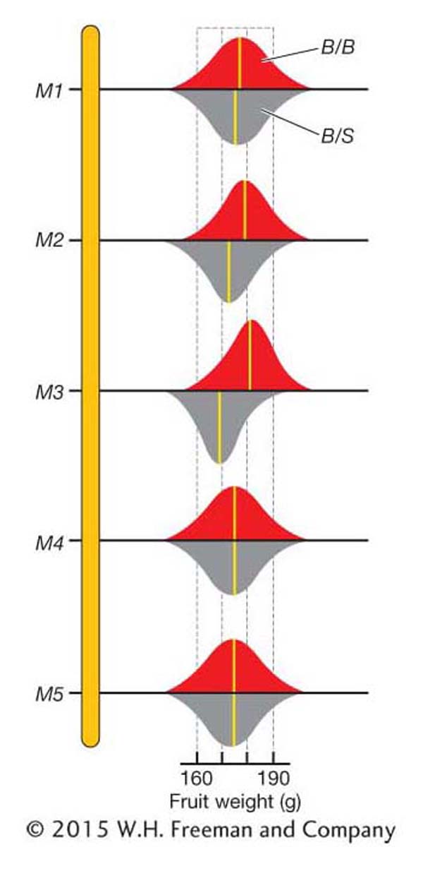
Figure 19-13 is a graphical representation of QTL-mapping data for many plants along one chromosome. The phenotypic data for the B/B and B/S genotypic classes are represented as frequency distributions so we can see the distributions of the trait values. At marker M1, the distributions are fully overlapping and the means for the B/B and B/S distributions are very close. It appears that the B/B and B/S classes have the same underlying distribution. At marker M3, the distributions are only partially overlapping and the means for the B/B and B/S distributions are quite different. The B/B and B/S classes have different underlying distributions similar to the situation in Figure 19-11. We have evidence for a QTL near M3.

As shown in Figure 19-13, the trait means for the B/B and B/S groups at some markers are nearly the same. At other markers, these means are rather different. How different do they need to be before we declare that a QTL is located near a marker? The statistical details for answering this question are beyond the scope of this text. However, let’s review the basic logic behind the statistics. The statistical analysis involves calculating the probability of observing the data (the specific fruit weights and marker-locus genotypes for all the plants) given that there is a QTL near the marker locus and the probability of observing the data given that there is not a QTL near the marker locus. The ratio of these two probabilities is called the “odds”:

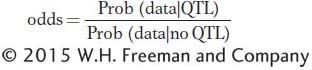
The vertical line | means “given,” and the term Prob(data|QTL) reads “the probability of observing the data given that there is a QTL.” If the probability of the data when there is a QTL is 0.1 and the probability of the data when there is no QTL is 0.001, then the odds are 0.1/0.001 = 100. That is, the odds are 100 to 1 in favor of there being a QTL. Researchers report the log₁₀ of the odds, or the Lod score. So, if the odds ratio is 100, then the log₁₀ of 100, or Lod score, is 2.0.

If there is a QTL near the marker, then the data were drawn from two underlying distributions—one distribution for the B/B class and one for the B/S class. Each of these distributions has its own mean and variance. If there is no QTL, then the data were drawn from a single distribution for which the mean and the variance are those of the entire BC₁ population. At marker locus M1 in Figure 19-13, the distributions for the B/B and B/S classes are nearly identical. Thus, there is a high probability that the data were drawn from a single underlying distribution. At marker M3, the distributions for the B/B and B/S classes are quite different. Thus, there is a higher probability of observing our data if we infer that the B/B plants were drawn from one distribution and B/S plants from another.

In addition to testing for QTL at the marker loci where the genotypes are known, Lod scores can be calculated for points between the markers. This can be done by using the genotypes of the flanking markers to infer the genotypes at points between the markers. For example, in Table 19-6, plant BC₁-001 is B/B at markers M1 and M2, and so it has a high probability of being B/B at all points in between. Plant BC₁-003 is B/B at marker M1 but B/S at M2, and so the plant might be either B/B or B/S at points in between. The odds equation incorporates this uncertainty when one calculates the Lod score at points between the markers.

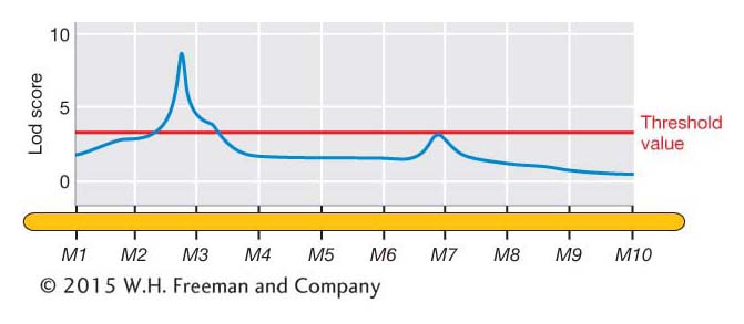
The Lod scores can be plotted along the chromosome as shown by the blue line in Figure 19-14. Such plots typically show some peaks of various heights as well as stretches that are relatively flat. The peaks represent putative QTL, but how high does a peak need to be before we declare that it represents a QTL? As discussed in Chapters 4 and 18, we can set a statistical threshold for rejecting the “null hypothesis.” In this case, the null hypothesis is that “there is not a QTL at a specific position along the chromosome.” The greater the Lod score, then the lower the probability under the null hypothesis. There are different statistical procedures for setting a “threshold value” for the Lod score. Where the Lod score exceeds the threshold value, then we reject the null hypothesis in favor of the alternative hypothesis that a QTL is located at that position. In Figure 19-14, the Lod score exceeds the threshold value (red line) near marker locus M3. We conclude that a QTL is located near M3.

746

In addition to backcross populations, QTL mapping can be done with F₂ populations and other breeding designs. An advantage of using an F₂ population is that one gets estimates of the mean trait values for all three QTL genotypes: homozygous parent-1, homozygous parent-2, and heterozygous. With these data, one can get estimates of the additive (A) and dominance (D) effects of the QTL as discussed earlier in this chapter. Thus, QTL mapping enables us to learn about gene action, whether dominant or additive, for each QTL.

Here is an example. Suppose we studied an F₂ population from a cross of Beef-master and Sungold tomatoes and we identified two QTL for fruit weight. The mean fruit weights for the different genotypic classes at the QTL might look something like this:

We can use these fruit weight values for the QTL to calculate the additive and dominance effects. QTL 1 is purely additive (D = 0), but QTL 2 has a large dominance effect. Also, notice that the additive effect of QTL 2 is more than 4 times that of QTL 1 (45 versus 10). Some QTL have large effects, and others have rather small effects.

What can be learned from QTL mapping? With the most powerful QTL-mapping designs, geneticists can estimate (1) the number of QTL (genes) affecting a trait, (2) the genomic locations of these genes, (3) the size of the effects of each QTL, (4) the mode of gene action for the QTL (dominant versus additive), and (5) whether one QTL affects the action of another QTL (epistatic interaction). In other words, one can get a rather complete description of the genetic architecture for the trait.

Much has been learned about genetic architecture from QTL-mapping studies in diverse organisms. Here are two examples. First, flowering time in maize is a classic quantitative or continuous trait. Flowering time is a trait of critical importance in maize breeding since the plants must flower and mature before the end of the growing season. Maize from Canada is adapted to flower within 45 days after planting, while maize from Mexico can require 120 days or longer. QTL mapping has shown that the genetic architecture for flowering time in maize involves more than 50 genes. Results from one experiment are shown in Figure 19-15a; these results show evidence for 15 QTL. QTL for maize flowering time generally have a small effect, such that substituting one allele for another at a QTL alters flowering time by only one day or less. Thus, the difference in flowering time between tropical and temperate maize involves many QTL.

747

Second, mice have been used to map QTL for many disease-susceptible traits. What one learns about disease-susceptibility genes in mice is often true in humans as well. Figure 19-15b shows the results of a genomic scan in mice for QTL for bone mineral density (BMD), the trait underlying osteoporosis. This scan identified two QTL, one on chromosome 9 and one on chromosome 12. From studies such as this, researchers have indentified over 80 QTL in mice that may contribute to susceptibility to osteoporosis. Similar studies have been done on dozens of other disease conditions.

QTL mapping does not typically reveal the identity of the gene(s) at the QTL. At its best, the resolution of QTL mapping is on the order of 1 to 10 cM, the size of a region that can contain 100 or more genes. To go from QTL to a single gene requires additional experiments to fine-map a QTL. To do this, the researcher creates a set of genetic homozygous stocks (also called lines), each with a crossover near the QTL. These stocks or lines differ from one another near the QTL, but they are identical to one another (isogenic) throughout the rest of their genomes. Lines that are identical throughout their genomes except for a small region of interest are called congenic or nearly isogenic lines. The isolation of QTL in an isogenic background is critical because only the single QTL region differs between the congenic lines. Thus, the use of congenic lines eliminates the complications caused by having multiple QTL segregate at the same time.

748

Using the tomato fruit weight example from above, the chromosome region for a set of such congenic lines is shown in Figure 19-16. The genes (flc, arf4,…) are shown at the top, and the location for each crossover is indicated by the switch in color from red (Beefmaster genotype) to yellow (Sungold genotype). The mean fruit weight for the congenic lines carrying these recombinant chromosomes is indicated on the right. By inspection of Figure 19-16, you’ll notice that all lines with the Beefmaster allele of kin1 (a kinase gene) have fruit of ∼180 g, while those with the Sungold allele of kin1 have fruit of about ∼170 g. None of the other genes are associated with fruit weight in this way. If confirmed by appropriate statistical tests, this result allows us to identify kin1 as the gene underlying this QTL.

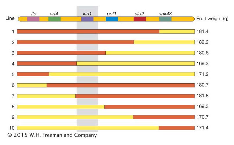
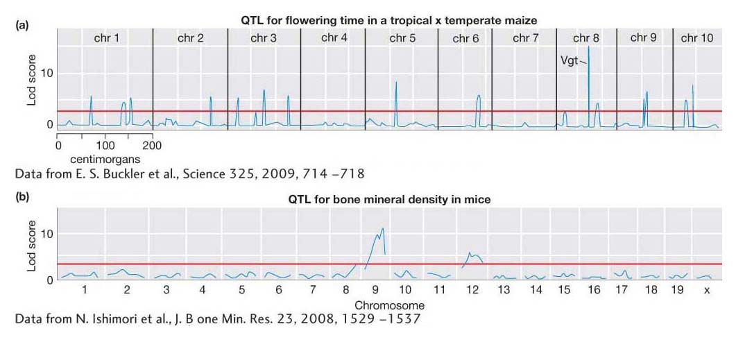
Table 19-7 lists a small sample of the hundreds of genes or QTL affecting quantitative variation from different species that have been identified. The list includes the gene for maize flowering time, Vgt, that underlies one of the Lod peaks in Figure 19-15a. One notable aspect of this list is the diversity of gene functions. There does not appear to be a rule that only particular types of genes can be a QTL. Most, if not all, genes in the genomes of organisms are likely to contribute to quantitative variation in populations.

749