Chapter 10: Inference for Regression

10.2 10.2 More Detail about Simple Linear Regression

When you complete this section, you will be able to:

• Construct a linear regression analysis of variance (ANOVA) table.
• Use an ANOVA table to perform the ANOVA F test and draw appropriate conclusions regarding H₀: β₁ = 0.
• Use an ANOVA table to compute the square of the sample correlation and provide an interpretation of it in terms of explained variation.
• Perform, using a calculator, inference in simple linear regression when a computer is not available.
• Distinguish the formulas for the standard error that we use for a confidence interval for the mean response and the standard error that we use for a prediction interval when x = x*.
• Test the hypothesis that there is no linear association in the population and summarize the results.
• Explain the close connection between the tests H₀: β₁ = 0 and H₀: ρ = 0.

In this section, we study three topics. The first is analysis of variance for regression. If you plan to read Chapter 11 on multiple regression, you should study this material. The second topic concerns computations for regression inference. The section we just completed assumes that you have access to software or a statistical calculator. Here we present and illustrate the use of formulas for the inference procedures. Finally, we discuss inference for correlation.

583

Analysis of variance for regression

The usual computer output for regression includes additional calculations called analysis of varianceanalysis of variance. Analysis of variance, often abbreviated ANOVA, is essential for multiple regression (Chapter 11) and for comparing several means (Chapters 12 and 13). Analysis of variance summarizes information about the sources of variation in the data. It is based on the

DATA = FIT + RESIDUAL

framework (page 560).

The total variation in the response y is expressed by the deviations . If these deviations were all 0, all observations would be equal and there would be no variation in the response. There are two reasons the individual observations are not all equal to their mean .

1. The responses correspond to different values of the explanatory variable x and will differ because of that. The fitted value estimates the mean response for . The differences reflect the variation in mean response due to differences in the . This variation is accounted for by the regression line because the ’s lie exactly on the line.
2. Individual observations will vary about their mean because of variation within the subpopulation of responses for a fixed x_i. This variation is represented by the residuals that record the scatter of the actual observations about the fitted line.

The overall deviation of any y observation from the mean of the y’s is the sum of these two deviations:

In terms of deviations, this equation expresses the idea that DATA = FIT + RESIDUAL.

Several times, we have measured variation by an average of squared deviations. If we square each of the preceding three deviations and then sum over all n observations, it can be shown that the sums of squares add:

We rewrite this equation as

SST = SSM + SSE

where

584

The SS in each abbreviation stands for sum of squares,sum of squares and the T, M, and E stand for total, model, and error, respectively. (“Error’’ here stands for deviations from the line, which might better be called “residual’’ or “unexplained variation.’’) The total variation, as expressed by SST, is the sum of the variation due to the straight-line model (SSM) and the variation due to deviations from this model (SSE). This partition of the variation in the data between two sources is the heart of analysis of variance.

If H₀: β₁ = 0 were true, there would be no subpopulations, and all of the y’s should be viewed as coming from a single population with mean μ_y. The variation of the y’s would then be described by the sample variance

The numerator in this expression is SST. The denominator is the total degrees of freedom, or simply DFT.

degrees of freedom, p. 40

Just as the total sum of squares SST is the sum of SSM and SSE, the total degrees of freedom DFT is the sum of DFM and DFE, the degrees of freedom for the model and for the error:

DFT = DFM + DFE

The model has one explanatory variable x, so the degrees of freedom for this source are DFM = 1. Because DFT = n − 1, this leaves DFE = n − 2 as the degrees of freedom for error.

For each source, the ratio of the sum of squares to the degrees of freedom is called the mean squaremean square, or simply MS. The general formula for a mean square is

Each mean square is an average squared deviation. MST is just , the sample variance that we would calculate if all of the data came from a single population. MSE is also familiar to us:

It is our estimate of σ², the variance about the population regression line.

SUMS OF SQUARES, DEGREES OF FREEDOM, AND MEAN SQUARES

Sums of squares represent variation present in the responses. They are calculated by summing squared deviations. Analysis of variance partitions the total variation between two sources.

The sums of squares are related by the formula

SST = SSM + SSE

That is, the total variation is partitioned into two parts, one due to the model and one due to deviations from the model.

585

Degrees of freedom are associated with each sum of squares. They are related in the same way:

DFT = DFM + DFE

To calculate mean squares, use the formula

In Section 2.4 (page 116), we noted that r²interpretation of r ² is the fraction of variation in the values of y that is explained by the least-squares regression of y on x. The sums of squares make this interpretation precise. Recall that SST = SSM + SSE. It is an algebraic fact that

Because SST is the total variation in y and SSM is the variation due to the regression of y on x, this equation is the precise statement of the fact that r² is the fraction of variation in y explained by x in the linear regression.

The ANOVA F test

The null hypothesis H₀: β₁ = 0 that y is not linearly related to x can be tested by comparing MSM with MSE. The ANOVA test statistic is an F statisticF statistic,

When H₀ is true, this statistic has an F distribution with 1 degree of freedom in the numerator and n − 2 degrees of freedom in the denominator. These degrees of freedom are those of MSM and MSE. When β₁ ≠ 0, MSM tends to be large relative to MSE. So, large values of F are evidence against H₀ in favor of the two-sided alternative.

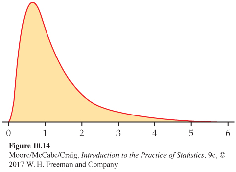
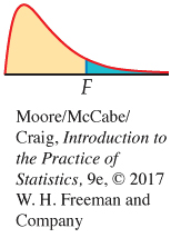
The F distributionsF distributions are a family of distributions with two parameters: the degrees of freedom of the mean square in the numerator and denominator of the F statistic. The F distributions are another of R. A. Fisher’s contributions to statistics and are called F in his honor. Fisher introduced F statistics for comparing several means. We meet these useful statistics in Chapters 14 and 15.

The numerator degrees of freedom are always mentioned first. Interchanging the degrees of freedom changes the distribution, so the order is important. Our brief notation will be F(j, k) for the F distribution with j degrees of freedom in the numerator and k in the denominator. The F distributions are not symmetric but are right-skewed. The density curve in Figure 10.14 illustrates the shape. Because mean squares cannot be negative, the F statistic takes only positive values, and the F distribution has no probability below 0. The peak of the F density curve is near 1; values much greater than 1 provide evidence against the null hypothesis.

We recommend using statistical software for calculations involving F distributions. We do, however, supply a table of critical values similar to Table D. Tables of F critical values are awkward because a separate table is needed for every pair of degrees of freedom j and k. Table E in the back of the book gives upper p critical values of the F distributions for p = 0.10, 0.05, 0.025, 0.01, and 0.001.

586

Figure 10.14: FIGURE 10.14 The density curve for the F(9,10) distribution. The F distributions are skewed to the right.

ANALYSIS OF VARIANCE F TEST

In the simple linear regression model, the hypotheses

H₀: β₁ = 0

H_a: β₁ ≠ 0

are tested by the F statistic

The P-value is the probability that a random variable having the F(1, n − 2) distribution is greater than or equal to the calculated value of the F statistic.

The F statistic tests the same null hypothesis as one of the t statistics that we encountered earlier in this chapter, so it is not surprising that the two are related. It is an algebraic fact that t² = F in this case. For linear regression with one explanatory variable, we prefer the t form of the test because it more easily allows us to test one-sided alternatives and is closely related to the confidence interval for β₁.

The ANOVA calculations are displayed in an analysis of variance table, often abbreviated ANOVA tableANOVA table. Here is the format of the table for simple linear regression:

Source	Degrees of freedom	Mean square	F
Model	1	SSM/DFM	MSM/MSE
Error	n − 2	SSE/DFE
Total	n − 1	SST/DFT

587

EXAMPLE 10.15

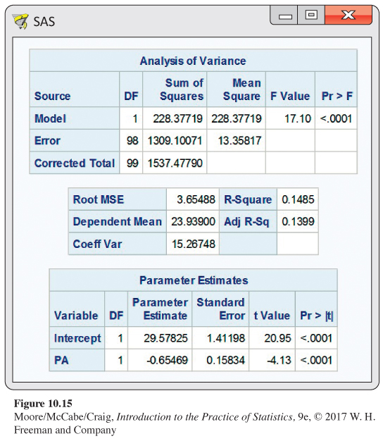
Interpreting SAS output for BMI and physical activity. The output generated by SAS for the physical activity study in Example 10.3 is given in Figure 10.15. Note that SAS uses the labels Model and Error but replaces Total with Corrected Total. Other statistical software packages may use slightly different labels. The F statistic is 17.10; the P-value is given as < 0.0001. There is strong evidence against the null hypothesis that there is no relationship between BMI and average number of steps per day (PA).

Figure 10.15: FIGURE 10.15 SAS output for the physical activity study, Example 10.15.

Now look at the output for the regression coefficients. The t statistic for PA is given as −4.13. If we square this number, we obtain the F statistic (accurate up to roundoff error). The value of r² is also given in the output. Average number of steps per day explains only 14.9% of the variability in BMI. Strong evidence against the null hypothesis that there is no relationship does not imply that a large percentage of the total variability is explained by the model.

USE YOUR KNOWLEDGE

Question 10.23

10.23 Reading linear regression outputs. Figure 10.4 (pages 562–564) shows the regression output from three other software packages and Excel. Create a table that lists the labels each output uses in its ANOVA table, the F statistic, its P-value, and r². Which of the outputs do you prefer? Explain your answer.

588

Calculations for regression inference

We recommend using statistical software for regression calculations. With time and care, however, the work is feasible with a calculator. We will use the following example to illustrate how to perform inference for regression analysis using a calculator.

EXAMPLE 10.16

Umbilical cord diameter and gestational age. Knowing the gestational age (GA) of a fetus is important for biochemical screening tests and planning for successful delivery. Typically GA is calculated as the number of days since the start of the woman’s last menstrual period (LMP). However, for women with irregular periods, GA is difficult to compute, and ultrasound imaging is often used. In the search for helpful ultrasound measurements, a group of Nigerian researchers looked at the relationship between umbilical cord diameter (mm) and gestational age based on LMP (weeks).⁸ Here is a small subset of the data:

Umbilical cord diameter (x)	2	6	9	14	21	23
Gestational age (y)	16	18	26	33	28	39

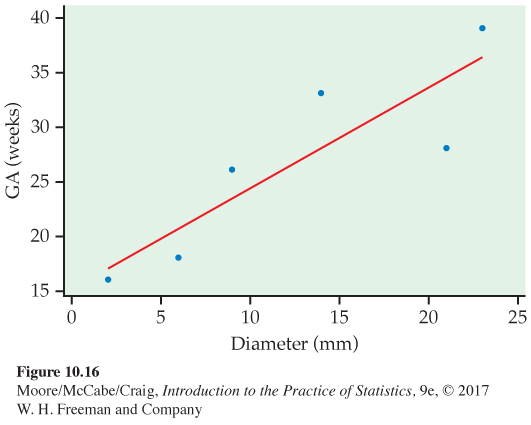
The data and the least-squares line are plotted in Figure 10.16. The strong straight-line pattern suggests that we can use linear regression to model the relationship between cord diameter and gestational age.

Figure 10.16: FIGURE 10.16 Scatterplot and regression line, Example 10.16.

We begin our regression calculations by fitting the least-squares line. Fitting the line gives estimates b₁ and b₀ of the model parameters β₁ and β₀. Next we examine the residuals from the fitted line and obtain an estimate s of the remaining parameter σ. These calculations are preliminary to inference. Finally, we use s to obtain the standard errors needed for the various interval estimates and significance tests. Roundoff errors that accumulate during these calculations can ruin the final results. Be sure to carry many significant digits and check your work carefully.

589

Preliminary calculations After examining the scatterplot (Figure 10.16) to verify that the data show a straight-line pattern, we begin our calculations.

EXAMPLE 10.17

Summary statistics for gestational age study. We start by making a table with the mean and standard deviation for each of the variables, the correlation, and the sample size. These calculations should be familiar from Chapters 1 and 2. Here is the summary:

Variable	Mean	Standard deviation	Correlation	Sample size
Diameter		s_x = 8.36062	r = 0.87699	n = 6
Gestational age		s_y = 8.75595

These quantities are the building blocks for our calculations.

We will need one additional quantity for the calculations to follow. It is the expression . We obtain this quantity as an intermediate step when we calculate s_x. You could also find it using the fact that . You should verify that the value for our example is

Our first task is to find the least-squares line. This is easy with the building blocks that we have assembled.

EXAMPLE 10.18

Computing the least-squares regression line. The slope of the least-squares line is

= 0.91846

The intercept is

= 26.66667 − (0.91846)(12.5)

= 15.18592

The equation of the least-squares regression line is therefore

This is the line shown in Figure 10.16.

We now have estimates of the first two parameters, β₀ and β₁, of our linear regression model. Next, we find the estimate of the third parameter, σ: the standard deviation s about the fitted line. To do this we need to find the predicted values and then the residuals.

590

EXAMPLE 10.19

Computing the predicted values and residuals. The first observation is a diameter of x = 2. The corresponding predicted value of gestational age is

= 15.1859 + (0.9185)(2)

= 17.023

and the residual is

= 16 − (17.023)

= −1.023

The residuals for the other diameters are calculated in the same way. They are −2.697, 2.548, 4.955, −6.474 and 2.689, respectively. Notice that the sum of these six residuals is zero (except for some roundoff error). When doing these calculations by hand, it is always helpful to check that the sum of the residuals is zero.

EXAMPLE 10.20

Computing s². The estimate of σ² is s², the sum of the squares of the residuals divided by n − 2. The estimated standard deviation about the line is the square root of this quantity.

= 22.127

So the estimate of the standard deviation about the line is

USE YOUR KNOWLEDGE

Question 10.24

10.24 Computing residuals. Refer to Examples 10.17, 10.18, and 10.19.

(a) Show that the least squares line goes through .

(b) Verify that the other five residuals are as stated in Example 10.19.

Inference for slope and intercept Confidence intervals and significance tests for the slope β₁ and intercept β₀ of the population regression line make use of the estimates b₁ and b₀ and their standard errors. Some algebra and the rules for variances establishes that the standard deviation of b₁ is

rules for variances, p. 258

591

Similarly, the standard deviation of b₀ is

To estimate these standard deviations, we need only replace σ by its estimate s.

STANDARD ERRORS FOR ESTIMATED REGRESSION COEFFICIENTS

The standard error of the slope b₁ of the least-squares regression line is

The standard error of the intercept b₀ is

The plot of the regression line with the data in Figure 10.16 shows a very strong relationship, but our sample size is small. We assess the situation with a significance test for the slope.

EXAMPLE 10.21

Testing the slope. First we need the standard error of the estimated slope:

= 0.2516

To test

H₀: β₁ = 0

H_a: β₁ ≠ 0

calculate the t statistic:

Using Table D with n − 2 = 4 degree of freedom, we conclude that 0.02 < P < 0.04. The exact P-value obtained from software is 0.022. The data provide evidence in favor of a linear relationship between gestational age and umbilical cord diameter (t = 3.65, df = 4, 0.02 < P < 0.04).

Two things are important to note about this example. First, it is important to remember that we need to have a very large effect if we expect to detect a slope different from zero with a small sample size. The estimated slope is more than 3.5 standard deviations away from zero, but we are not much below the 0.05 standard for statistical significance. Second, because we expect gestational age to increase with increasing diameter, a one-sided significance test would be justified in this setting.

592

The significance test tells us that the data provide sufficient information to conclude that gestational age and umbilical cord diameter are linearly related. We use the estimate b₁ and its confidence interval to further describe the relationship.

EXAMPLE 10.22

Computing a 95% confidence interval for the slope. Let’s find a 95% confidence interval for the slope β₁. The degrees of freedom are n − 2 = 4, so t* from Table D is 2.776. We compute

= 0.9185 ± 0.6984

The interval is (0.220, 1.617). For each additional millimeter in diameter, the gestational age of the fetus is expected to be 0.220 to 1.617 weeks older.

In this example, the intercept β₀ does not have a meaningful interpretation. An umbilical cord diameter of zero millimeters is not realistic. For problems where inference for β₀ is appropriate, the calculations are performed in the same way as those for β₁. Note that there is a different formula for the standard error, however.

Confidence intervals for the mean response and prediction intervals for a future observation When we substitute a particular value x* of the explanatory variable into the regression equation and obtain a value of we can view the result in two ways:

1. We have estimated the mean response μ_y.
2. We have predicted a future value of the response y.

The margins of error for these two uses are often quite different. Prediction intervals for an individual response are wider than confidence intervals for estimating a mean response. We now proceed with the details of these calculations. Once again, standard errors are the essential quantities. And once again, these standard errors are multiples of s, our basic measure of the variability of the responses about the fitted line.

STANDARD ERRORS FOR AND

The standard error of is

The standard error for predicting an individual response is

593

Note that the only difference between the formulas for these two standard errors is the extra 1 under the square root sign in the standard error for prediction. This standard error is larger due to the additional variation of individual responses about the mean response. This additional variation remains regardless of the sample size n and is the reason that prediction intervals are wider than the confidence intervals for the mean response.

For the gestational age example, we can think about the average gestational age for a particular subpopulation, defined by the umbilical cord diameter. The confidence interval would provide an interval estimate of this subpopulation mean. On the other hand, we might want to predict the gestational age for a new fetus. A prediction interval attempts to capture this new observation.

EXAMPLE 10.23

Computing a confidence interval for m. Let’s find a 95% confidence interval for the average gestational age when the umbilical cord diameter is 10 millimeters. The estimated mean age is

= 15.1859 + (0.9185)(10)

= 24.371

The standard error is

= 2.021

To find the 95% confidence interval, we compute

= 24.371 ± 5.610

The interval is 18.761 to 29.981 weeks of age. This is a pretty wide interval given gestation lasts for about 40 weeks.

Calculations for the prediction intervals are similar. The only difference is the use of the formula for in place of . This results in a much wider interval. In fact, the interval is slightly more than 28 weeks in width. Even though a linear relationship was found statistically significant, it does not appear umbilical cord diameter is a precise predictor of gestational age.

Inference for correlation

The correlation coefficient is a measure of the strength and direction of the linear association between two variables. Correlation does not require an explanatory-response relationship between the variables. We can consider the sample correlation r as an estimate of the correlation in the population and base inference about the population correlation on r.

correlation, p. 101

594

The correlation between the variables x and y when they are measured for every member of a population is the population correlationpopulation correlation. As usual, we use Greek letters to represent population parameters. In this case ρ (the Greek letter rho) is the population correlation.

When ρ = 0, there is no linear association in the population. In the important case where the two variables x and y are both Normally distributed, the condition ρ = 0 is equivalent to the statement that x and y are independent. That is, there is no association of any kind between x and y. (Technically, the condition required is that x and y be jointly Normal variablesjointly Normal variables. This means that the distribution of x is Normal and also that the conditional distribution of y, given any fixed value of x, is Normal.) We, therefore, may wish to test the null hypothesis that a population correlation is 0.

TEST FOR A ZERO POPULATION CORRELATION

To test the hypothesis H₀: ρ = 0, compute the t statistic

where n is the sample size and r is the sample correlation.

In terms of a random variable T having the t(n − 2) distribution, the P-value for a test of H₀ against

H_a: ρ > 0 is P(T ≥ t)

H_a: ρ < 0 is P(T ≤ t)

H_a: ρ ≠ 0 is 2P(T ≥ |t|)

Most computer packages have routines for calculating correlations, and some will provide the significance test for the null hypothesis that ρ is zero.

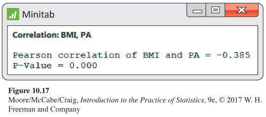
EXAMPLE 10.24

Correlation in the physical activity study. The Minitab output for the physical activity example appears in Figure 10.17. The sample correlation between BMI and the average number of steps per day (PA) is r = −0.385. Minitab calls this a Pearson correlation to distinguish it from other kinds of correlations that it can calculate. The P-value for a two-sided test of H₀: ρ = 0 is given as 0.000. This means that the actual P-value is less than 0.0005. We conclude that there is a nonzero correlation between BMI and PA.

595

Figure 10.17: FIGURE 10.17 Minitab output for the physical activity study, Example 10.24.

If we wanted to test the one-sided alternative that the population correlation is negative, we divide the P-value in the output by 2, after checking that the sample coefficient is in fact negative.

If your software does not give the significance test, you can do the computations easily with a calculator.

EXAMPLE 10.25

Correlation test using a calculator. The correlation between BMI and PA is r = −0.385. Recall that n = 100. The t statistic for testing the null hypothesis that the population correlation is zero is

= −4.13

The degrees of freedom are n − 2 = 98. From Table D, we conclude that P < 0.0001. This agrees with the Minitab output in Figure 10.17, where the P-value is given as 0.000. The data provide clear evidence that BMI and PA are related.

There is a close connection between the significance test for a correlation and the test for the slope in a linear regression. Recall that

From this fact, we see that if the slope is 0, so is the correlation, and vice versa. It should come as no surprise to learn that the procedures for testing H₀: β₁ = 0 and H₀: ρ = 0 are also closely related. In fact, the t statistics for testing these hypotheses are numerically equal. That is,

Check that this holds in both of our examples.

In our examples, the conclusion that there is a statistically significant correlation between the two variables would not come as a surprise to anyone familiar with the meaning of these variables. The significance test simply tells us whether or not there is evidence in the data to conclude that the population correlation is different from 0. The actual size of the correlation is of considerably more interest. We would, therefore, like to give a confidence interval for the population correlation. Unfortunately, most software packages do not perform this calculation. Because hand calculation of the confidence interval is very tedious, we do not give the method here.⁹