13.5 What’s wrong? In each of the following, identify what is wrong and then either explain why it is wrong or change the wording of the statement to make it true.

13.6 Is there an interaction? Each of the following tables gives means for a two-way ANOVA. Make a plot of the means with the levels of Factor A on the x axis. State whether or not there is an interaction, and if there is, describe it.

13.7 Describing a two-way ANOVA model. A 3 × 3 ANOVA was run with four observations per cell.

13.8 Determining the critical value of F. For each of the following situations, state how large the F statistic needs to be for rejection of the null hypothesis at the 5% level. Sketch each distribution and indicate the region where you would reject.

13.9 Identifying the factors of a two-way ANOVA model. For each of the following situations, identify both factors and the response variable. Also, state the number of levels for each factor (I and J) and the total number of observations (N).

13.10 Determining the degrees of freedom. For each part in Exercise 13.9, outline the ANOVA table, giving the sources of variation and the degrees of freedom.

13.11 Smart shopping carts. Smart shopping carts are shopping carts equipped with scanners that track the total price of the items in the cart (real-time feedback). To help understand the smart shopping cart’s influence on spending behavior, a group of researchers designed a two-factor study. Each participant was randomly assigned to either be on or not on a budget of $35. Also, each participant’s cart was equipped with or without real-time feedback. The total amount spent on a common grocery list was the response.⁷

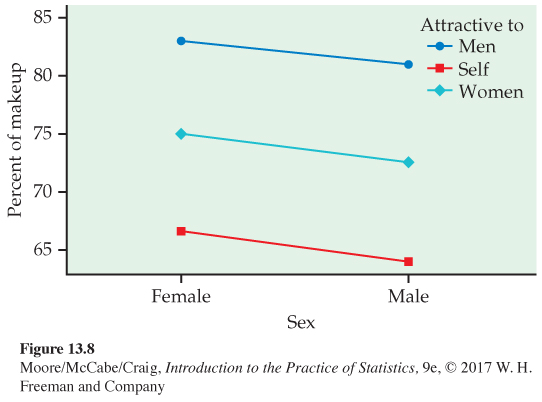
13.12 Using makeup. A study was performed in which 44 women participated as models. Each model was photographed after applying makeup as if she was going on a “night out.’’ Software was then used to create a sequence of 21 images ranging from 50% makeup to 150% makeup. Another set of observers (consisting of both sexes) was asked to look at each sequence of images and select the image that they felt was most attractive, what they felt was most attractive to other women, and what they felt was most attractive to other men. The average percent makeup over the 44 models was the response. Figure 13.8 replicates one of the plots used in their summary.⁸

13.13 Writing about testing worries and exam performance. For many students, self-induced worries and pressure to perform well on exams cause them to perform below their ability. This is because these worries compete with the working memory available for performance. Expressive writing has been shown to be an effective technique to overcome traumatic or emotional experiences. Thus, a group of researchers decided to investigate whether expressive writing prior to test-taking may help performance.⁹

The small study involved 20 subjects. Half the subjects were assigned to the expressive-writing group and the others to a control group. Each subject took two short mathematics exams. Prior to the first exam, students were told just to perform their best. Prior to the second exam, students were told that they each had been paired with another student and if the members of a pair both performed well on the exam, the pair would receive a monetary reward. Each student was then told privately that his or her partner had already scored well. This was done to create a high-stakes testing environment for the second exam. Those in the control group sat quietly for 10 minutes prior to taking the second exam. Those in the expressive-writing group had 10 minutes to write about their thoughts and feelings regarding the exam. The following table summarizes the test results (% correct):

13.14 Influence of age and sex on motor performance. The slowing of motor performance as humans age is well established. Differences across the sexes, however, are less so. A recent study assessed the motor performance of 246 healthy adults.¹⁰ One task was to tap the thumb and forefinger of the right hand together 20 times as quickly as possible. The following table summarizes the results (in seconds) for seven age classes and two sexes:

Generate a plot to look at changes in the time across age class for each sex. Describe what you see in terms of the main effects for age and sex as well as their interaction.

13.15 Influence of age and sex on motor performance, continued. Refer to the previous exercise.

13.16 Ecological effects of pharmaceuticals on fish. Drugs used to treat anxiety persist in wastewater effluent, resulting in relatively high concentrations of these drugs in our rivers and streams. To understand the impacts of these anxiety drugs on fish, researchers commonly expose fish to various levels of a drug in a laboratory setting and observe their behavior.¹¹ In one 2 × 2 experiment, researchers considered exposure to oxazepan through the water (Y/N) and through the diet (Y/N). Ten one-year-old perch were assigned to each of the four treatment combinations. After seven days of exposure, each fish was observed for activity. This was recorded as the number of swimming bouts (defined as movement exceeding 3.5 cm) over a 10-minute period.

13.17 Where are your eyes? The objectifying gaze, often referred to as “ogling’’ or “checking out,’’ can have have many adverse consequences. A group of researchers used eye-tracking technology to better understand the nature and causes for this gaze. They asked 29 women and 36 men to look at images of college-aged women. Each woman had the same clothes and neutral expression but varied in body shape (ideal, average, and below average). Prior to looking at the images, each participant was told to focus on either the appearances or personalities of the women. Here is a summary of the amount of time (in milliseconds) the eyes focused on the chest of the women:¹²

13.18 Ecological effects of pharmaceuticals on fish, continued. Refer to Exercise 13.16.

13.19 The influences of transaction history and a thank-you statement. A service failure is defined as any service-related problem (real or perceived) that transpires during a customer’s experience with a firm. In the hotel industry, there is a high human component, so these sorts of failures commonly occur regardless of extensive training and established policies. As a result, hotel firms must learn to effectively react to these failures. A recent study investigated the relationship between a consumer’s transaction history (levels: long and short) and an employee thank-you statement (levels: yes and no) on a consumer’s repurchase intent.¹³ Each subject was randomly assigned to one of the four treatment groups and asked to read some service failure/resolution scenarios and respond accordingly. Repurchase intent was measured using a nine-point scale. Here is a summary of the means:

13.20 Transaction history and a thank-you statement, continued. Refer to the previous exercise. The numbers of subjects in the cells were not equal, so the researchers used linear regression to analyze the data. This was done by creating an indicator variable for each factor and the interaction. Following is a partial ANOVA table. Complete it and state your conclusions regarding the main effects and interaction described in the previous exercise.

13.21 The effects of proximity and visibility on food intake. A study investigated the influence that proximity and visibility of food have on food intake.¹⁴ A total of 40 secretaries from the University of Illinois participated in the study. A candy dish full of individually wrapped chocolates was placed either at the desk of the participant or at a location 2 meters from the participant. The candy dish was either a clear (candy visible) or opaque (candy not visible) covered bowl. After a week, the researchers noted not only the number of candies consumed per day, but also the self-reported number of candies consumed by each participant. The following table summarizes the mean difference between these two values (reported minus actual):

13.22 Bilingualism. Not only does speaking two languages have many practical benefits in this globalized world, but there is also growing evidence that it appears to help with brain functioning as we age. In one study, 80 participants were divided equally among 4 groups: younger adult bilinguals, older adult bilinguals, younger adult monolinguals, and older adult monolinguals.¹⁵ Each participant was asked to complete a series of color-shape task-switching tests. For our analysis, we’ll focus on the total reaction time (in microseconds) for these experiments. The shorter the reaction time, the better.

13.23 Bilingualism, continued. Refer to the previous exercise.

13.24 Hypotension and endurance exercise. In sedentary individuals, low blood pressure (hypotension) often occurs after a single bout of aerobic exercise and lasts nearly two hours. This can cause dizziness, light-headedness, and possibly fainting upon standing. It is thought that endurance exercise training can reduce the degree of postexercise hypotension. To test this, researchers studied 16 endurance-trained and 16 sedentary men and women.¹⁶ The following table summarizes the postexercise systolic arterial pressure (mm Hg) after 60 minutes of upright cycling:

13.25 The effect of humor. In advertising, humor is often used to overcome sales resistance and stimulate customer purchase behavior. One experiment looked at the use of humor to offset the negative feelings often associated with website encounters.¹⁷ The setting of the experiment was an online travel agency, and the researchers used a three-factor design, each factor with two levels. The factors were humor (used, not used), process (favorable, unfavorable), and outcome (favorable, unfavorable). For the humor condition, cartoons and jokes of the day about skiing were presented on the site. For the no humor condition, standard pictures of ski sites were used. Two hundred and forty-one business students from a large Dutch university participated in the experiment. Each was randomly assigned to one of the eight treatment conditions. The students were asked to book a skiing holiday and then rate their perceived enjoyment and satisfaction with the process. All responses were measured on a seven-point Likert scale. A summary of the results for satisfaction follows:

13.26 Pooling the standard deviations. Refer to the previous exercise. Find the pooled estimate of the standard deviation for these data. What are its degrees of freedom? Using the rule from Chapter 12 (page 654), is it reasonable to use a pooled standard deviation for the analysis? Explain your answer.

13.27 Describing the effects. Refer to Exercise 13.25. The P-values for all main effects and two-factor interactions are significant at the 0.05 level. Using the table, find the marginal means (that is, the mean for the no humor treatment, the mean for the no humor and unfavorable process treatment combination, etc.) and use them to describe these effects.

13.28 Acceptance of functional foods. Functional foods are foods that are fortified with health-promoting supplements, like calcium-enriched orange juice or vitamin-enriched cereal. Although the number of functional foods is growing in the marketplace, very little is known about how the next generation of consumers views these foods. Because of this, a questionnaire was given to college students from the United States, Canada, and France.¹⁸ This questionnaire measured the students’ attitudes and beliefs about general food and functional food. One of the response variables collected concerned cooking enjoyment. This variable was the average of numerous items, each measured on a 10-point scale, where 1 = most negative value and 10 = most positive value. Here are the means:

13.29 Estimating the within-group variance. Refer to the previous exercise. Here are the cell standard deviations and sample sizes for cooking enjoyment:

Find the pooled estimate of the standard deviation for these data. Use the rule for examining standard deviations in ANOVA from Chapter 12 (page 654) to determine if it is reasonable to use a pooled standard deviation for the analysis of these data.

13.30 Comparing the groups. Refer to Exercises 13.28 and 13.29. The researchers presented a table of means with different superscripts indicating pairs of means that differed at the 0.05 significance level, using the Bonferroni method.

13.31 More on acceptance of functional foods. Refer to Exercise 13.28. The means for four of the response variables associated with functional foods are as follows:

For each of the four response variables, give a graphical summary of the means. Use this summary to discuss any interactions that are evident. Write a short report summarizing any differences in culture and sex with respect to the response variables measured.

13.32 Interpreting the results. The goal of the study in the previous exercise was to understand cultural and sex differences in functional food attitudes and behaviors among young adults, the next generation of food consumers. The researchers used a sample of undergraduate students and had each participant fill out the survey during class time. How reasonable is it to generalize these results to the young adult population in these countries? Explain your answer.

13.33 What can you conclude? Analysis of data for a 3 × 3 ANOVA with three observations per cell gave the F statistics in the following table:

What can you conclude from the information given?

13.34 What can you conclude? A study reported the following results for data analyzed using the methods that we studied in this chapter:

13.35 Conspicuous consumption and men’s testosterone levels. It is argued that conspicuous consumption is a means by which men communicate their social status to prospective mates. One study looked at changes in a male’s testosterone level in response to fluctuations in his status created by the consumption of a product.¹⁹ The products considered were a new and luxurious sports car and an old family sedan. Participants were asked to drive on either an isolated highway or a busy city street. A table of cell means and standard deviations for the change (post minus pre) in testosterone level follows:

13.36 The effects of peer pressure on mathematics achievement. Researchers were interested in comparing the relationship between high achievement in mathematics and peer pressure across several countries.²⁰ They hypothesized that in countries where high achievement is not valued highly, considerable peer pressure may exist. A questionnaire was distributed to 14-year-olds from three countries (Germany, Canada, and Israel). One of the questions asked students to rate how often they fear being called a nerd or teacher’s pet on a four-point scale (1 = never, 4 = frequently). The following table summarizes the response:

13.37 The effect of chromium on insulin metabolism. The amount of chromium in the diet has an effect on the way the body processes insulin. In an experiment designed to study this phenomenon, four diets were fed to male rats. There were two factors. Chromium had two levels: low (L) and normal (N). The rats were allowed to eat as much as they wanted (M), or the total amount that they could eat was restricted (R). We call the second factor Eat. One of the variables measured was the amount of an enzyme called GITH.²¹ The means for this response variable appear in the following table:

13.38 Use of animated agents in a multimedia environment. Multimedia learning environments are designed to enhance learning by providing a more hands-on and exploratory investigation of a topic. Often, animated agents (human-like characters) are used with the hope of enhancing social interaction with the software and thus improving learning. One group of researchers decided to investigate whether the presence of an agent and the type of verbal feedback provided were actually helpful.²² To do this, they recruited 135 college students and randomly divided them among four groups: agent/simple feedback, agent/elaborate feedback, no agent/simple feedback, and no agent/elaborate feedback. The topic of the software was thermodynamics. The change in score on a 20-question test taken before and after using the software was the response.

13.39 Trust of individuals and groups. Trust is an essential element in any exchange of goods or services. The following trust game is often used to study trust experimentally:

A sender starts with $X and can transfer any amount x ≤ X to a responder. The responder then gets $3x and can transfer any amount y ≤ 3x back to the sender. The game ends with final amounts X − x + y and 3x − y for the sender and responder, respectively.

The value x is taken as a measure of the sender’s trust, and the value y/3x indicates the responder’s trustworthiness. A recent study used this game to study the dynamics between individuals and groups of three.²³ The following table summarizes the average amount x sent by senders starting with $100:

13.40 Does the type of cooking pot affect iron content? Iron-deficiency anemia is the most common form of malnutrition in developing countries, affecting about 50% of children and women and 25% of men. Iron pots for cooking foods had traditionally been used in many of these countries, but they have been largely replaced by aluminum pots, which are cheaper and lighter. Some research has suggested that food cooked in iron pots will contain more iron than food cooked in other types of pots. One study designed to investigate this issue compared the iron content of some Ethiopian foods cooked in aluminum, clay, and iron pots.²⁴ Foods considered were yesiga wet’, beef cut into small pieces and prepared with several Ethiopian spices; shiro wet’, a legume-based mixture of chickpea flour and Ethiopian spiced pepper; and ye-atkilt allych’a, a lightly spiced vegetable casserole. Four samples of each food were cooked in each type of pot. The iron in the food is measured in milligrams of iron per 100 grams of cooked food. The data are shown in Table 13.1.

13.41 Interpreting the results. Refer to the previous exercise. Although there is a statistically significant interaction, do you think that these data support the conclusion that foods cooked in iron pots contain more iron than foods cooked in aluminum or clay pots? Discuss.

13.42 Analysis using a one-way ANOVA. Refer to Exercise 13.40. Rerun the analysis as a one-way ANOVA with nine groups and four observations per group. Report the results of the F test. Examine differences in means using a multiple-comparisons procedure. Summarize your results and compare them with those you obtained in Exercise 13.40.

13.43 Examination of a drilling process. One step in the manufacture of large engines requires that holes of very precise dimensions be drilled. The tools that do the drilling are regularly examined and are adjusted to ensure that the holes meet the required specifications. Part of the examination involves measurement of the diameter of the drilling tool. A team studying the variation in the sizes of the drilled holes selected this measurement procedure as a possible cause of variation in the drilled holes. They decided to use a designed experiment as one part of this examination. Some of the data are given in Table 13.2. The diameters in millimeters (mm) of five tools were measured by the same operator at three times (8:00 A.M., 11:00 A.M., and 3:00 P.M.). Three measurements were taken on each tool at each time. The person taking the measurements could not tell which tool was being measured, and the measurements were taken in random order.²⁵

13.44 Examination of a drilling process, continued. Refer to the previous exercise. Multiply each measurement by 0.04 to convert from millimeters to inches. Redo the plots and rerun the ANOVA using the transformed measurements. Summarize what parts of the analysis have changed and what parts have remained the same.

13.45 Do left-handed people live shorter lives than right-handed people? A study of this question examined a sample of 949 death records and contacted next of kin to determine handedness.²⁶ Note that there are many possible definitions of “left-handed.’’ The researchers examined the effects of different definitions on the results of their analysis and found that their conclusions were not sensitive to the exact definition used. For the results presented here, people were defined to be right-handed if they wrote, drew, and threw a ball with the right hand. All others were defined to be left-handed. People were classified by sex (female or male) and handedness (left or right), and a 2 × 2 ANOVA was run with the age at death as the response variable. The F statistics were 22.36 (handedness), 37.44 (sex), and 2.10 (interaction). The following marginal mean ages at death (in years) were reported: 77.39 (females), 71.32 (males), 75.00 (right-handed), and 66.03 (left-handed).

13.46 A radon exposure study. Scientists believe that exposure to the radioactive gas radon is associated with some types of cancers in the respiratory system. Radon from natural sources is present in many homes in the United States. A group of researchers decided to study the problem in dogs because dogs get similar types of cancers and are exposed to environments similar to those of their owners. Radon detectors are available for home monitoring, but the researchers wanted to obtain actual measures of the exposure of a sample of dogs. To do this, they placed the detectors in holders and attached them to the collars of the dogs. One problem was that the holders might, in some way, affect the radon readings. The researchers, therefore, devised a laboratory experiment to study the effects of the holders. Detectors from four series of production were available, so they used a two-way ANOVA design (series with four levels and holder with two, representing the presence or absence of a holder). All detectors were exposed to the same radon source and the radon measure in picocuries per liter was recorded.²⁷ The F statistic for the effect of series is 7.02, for holder it is 1.96, for the interaction it is 1.24, and N = 69.

13.47 A comparison of plant species under low water conditions. The PLANTS1 data file gives the percent of nitrogen in four different species of plants grown in a laboratory. The species are Leucaena leucocephala, Acacia saligna, Prosopis juliflora, and Eucalyptus citriodora. The researchers who collected these data were interested in commercially growing these plants in parts of the country of Jordan where there is very little rainfall. To examine the effect of water, they varied the amount per day from 50 millimeters (mm) to 650 mm in 100 mm increments. There were nine plants per species-by-water combination. Because the plants are to be used primarily for animal food, with some parts that can be consumed by people, a high nitrogen content is very desirable.

13.48 Examination of the residuals. Refer to the previous exercise. Examine the residuals. Are there any unusual patterns or outliers? If you think that there are one or more points that are somewhat extreme, rerun the two-way analysis without these observations. Does this change the results in any substantial way?

13.49 Analysis using multiple one-way ANOVAs. Refer to Exercise 13.47. Run a separate one-way analysis of variance for each water level. If there is evidence that the species are not all the same, use a multiple-comparisons procedure to determine which pairs of species are significantly different. In what way, if any, do the differences appear to vary by water level? Write a short summary of your conclusions.

13.50 More on the analysis using multiple one-way ANOVAs. Refer to Exercise 13.47. Run a separate one-way analysis of variance for each species and summarize the results. Because the amount of water is a quantitative factor, we can also analyze these data using regression. Run simple linear regressions separately for each species to predict nitrogen percent from water. Use plots to determine whether or not a line is a good way to approximate this relationship. Summarize the regression results and compare them with the one-way ANOVA results.

13.51 Another comparison of plant species under low water conditions. Refer to Exercise 13.47. Additional data collected by the same researchers according to a similar design are given in the PLANTS2 data file. Here, there are two response variables. They are fresh biomass and dry biomass. High values for both of these variables are desirable. The same four species and seven levels of water are used for this experiment. Here, however, there are four plants per species-by-water combination. Analyze each of the response variables in the PLANTS2 data file using the outline from Exercise 13.47.

13.52 Examination of the residuals. Perform the tasks described in Exercise 13.48 for the two response variables in the PLANTS2 data set.

13.53 Analysis using multiple one-way ANOVAs. Perform the tasks described in Exercise 13.49 for the two response variables in the PLANTS2 data set.

13.54 More on the analysis using multiple one-way ANOVAs. Perform the tasks described in Exercise 13.50 for the two response variables in the PLANTS2 data set.

13.55 Are insects more attracted to male plants? Some scientists wanted to determine if there are sex-related differences in the level of herbivory for the jack-in-the-pulpit, a spring-blooming perennial plant common in deciduous forests. A study was conducted in southern Maryland in forests associated with the Smithsonian Environmental Research Center (SERC).²⁸ To determine the effects of flowering and floral characteristics on herbivory, the researchers altered the floral morphology of male and female plants. The three levels of floral characteristics were (1) the spathes were completely removed; (2) in females, a gap was created in the base of the spathe, and in males, the gap was closed; (3) plants were not altered (control). The percent of leaf area damaged by thrips (an order of insects) between early May and mid-June was recorded for each of 30 plants per combination of sex and floral characteristic. Here is a table of means and standard deviations (in parentheses):

13.56 Change-of-majors study: HSS. Refer to the data given for the change-of-majors study in the data file MAJORS. Consider sex and whether the students changed majors as the two factors. Analyze the data for HSS, the high school science grades. Your analysis should include a table of sample sizes, means, and standard deviations; Normal quantile plots; a plot of the means; and a two-way ANOVA using sex and major as the factors. Write a short summary of your conclusions.

13.57 Change-of-majors study: HSE. Refer to the previous exercise. Analyze the data for HSE, the high school English grades. Your analysis should include a table of sample sizes, means, and standard deviations; Normal quantile plots; a plot of the means; and a two-way ANOVA using sex and major as the factors. Write a short summary of your conclusions.

13.58 Change-of-majors study: GPA. Refer to Exercise 13.56. Analyze the data for GPA, the college grade point average. Your analysis should include a table of sample sizes, means, and standard deviations; Normal quantile plots; a plot of the means; and a two-way ANOVA using sex and major as the factors. Write a short summary of your conclusions.

13.59 Change-of-majors study: SATV. Refer to Exercise 13.56. Analyze the data for SATV, the SAT Verbal score. Your analysis should include a table of sample sizes, means, and standard deviations; Normal quantile plots; a plot of the means; and a two-way ANOVA using sex and major as the factors. Write a short summary of your conclusions.

13.60 Search the Internet. Search the Internet or your library to find a study that is interesting to you and uses a two-way ANOVA to analyze the data. First describe the question or questions of interest, and then give the details of how ANOVA was used to provide answers. Be sure to include how the study authors examined the assumptions for the analysis. Evaluate how well the authors used ANOVA in this study. If your evaluation finds the analysis deficient, make suggestions for how it could be improved.