4.1 4.1 Randomness
When you complete this section, you will be able to:
• Identify random phenomena.
• Interpret the term probability for particular examples.
• Identify trials as independent or not.
216
Toss a coin, or choose a simple random sample (SRS). The result can’t be predicted in advance because the result will vary when you toss the coin or choose the sample repeatedly. But there is, nonetheless, a regular pattern in the results, a pattern that emerges clearly only after many repetitions. This remarkable fact is the basis for the idea of probability.
EXAMPLE 4.1
Toss a coin 5000 times. When you toss a coin, there are only two possible outcomes, heads or tails. Figure 4.1 shows the results of tossing a coin 5000 times twice (Trial A and Trial B). For each number of tosses from 1 to 5000, we have plotted the proportion of those tosses that gave a head.
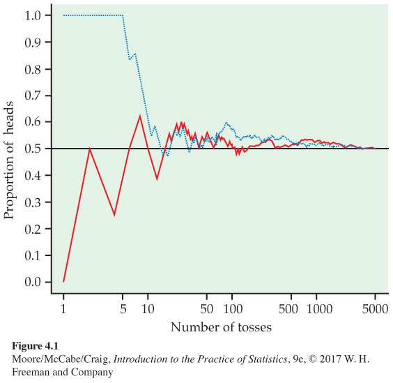
Trial A (red line) begins tail, head, tail, tail. You can see that the proportion of heads for Trial A starts at 0 on the first toss, rises to 0.5 when the second toss gives a head, then falls to 0.33 and 0.25 as we get two more tails. Trial B (blue dotted line), on the other hand, starts with five straight heads, so the proportion of heads is 1 until the sixth toss.
The proportion of tosses that produce heads is quite variable at first. Trial A starts low and Trial B starts high. As we make more and more tosses, however, the proportion of heads for each trial gets close to 0.5 and stays there.
If we made yet a third trial at tossing the coin a great many times, the proportion of heads would again settle down to 0.5 in the long run. We say that 0.5 is the probabilityprobability of a head. The probability 0.5 appears as a horizontal line on the graph.
217
![]()
The Probability applet on the text website animates Figure 4.1. It allows you to choose the probability of a head and simulate any number of tosses of a coin with that probability. Try it. You will see that the proportion of heads gradually settles down close to the chosen probability. Equally important, you will also see that the proportion in a small or moderate number of tosses can be far from this probability. Probability describes only what happens in the long run. Most people expect chance outcomes to show more short-term regularity than is actually true.
![]()
EXAMPLE 4.2
Significance testing and Type I errors. In Chapter 6, we will learn about significance testing and Type I errors. When we perform a significance test, we have the possibility of making a Type I error under certain circumstances. The significance-testing procedure is set up so that the probability of making this kind of error is small, usually 5%. If we perform a large number of significance tests under this set of circumstances, the proportion of times that we will make a Type I error is 0.05.
In the coin toss setting, the probability of a head is a characteristic of the coin being tossed. A coin is called fairfair coin if the probability of a head is 0.5; that is, it is equally likely to come up heads or tails. If we toss a coin five times and it comes up heads for all five tosses, we might suspect that the coin is not fair. Is this outcome likely if, in fact, the coin is fair? This is what happened in Trials A and B of Example 4.1. We will learn a lot more about significance testing in later chapters. For now, we are content with some very general ideas.
When the Type I error of a statistical significance procedure is set at 0.05, this probability is a characteristic of the procedure. If we roll a pair of dice once, we do not know whether the sum of the faces will be seven or not. Similarly, if we perform a significance test once, we do not know if we will make a Type I error or not. However, if the procedure is designed to have a Type I error probability of 0.05, then we are much less likely than not to make a Type I error.
The language of probability
“Random” in statistics is not a synonym for “unpredictable” but a description of a kind of order that emerges in the long run. We often encounter the unpredictable side of randomness in our everyday experience, but we rarely see enough repetitions of the same random phenomenon to observe the long-term regularity that probability describes. You can see that regularity emerging in Figure 4.1. In the very long run, the proportion of tosses that give a head is 0.5. This is the intuitive idea of probability. Probability 0.5 means “occurs half the time in a very large number of trials.”
RANDOMNESS AND PROBABILITY
We call a phenomenon random if individual outcomes are uncertain but there is, nonetheless, a regular distribution of outcomes in a large number of repetitions.
The probability of any outcome of a random phenomenon is the proportion of times the outcome would occur in a very long series of repetitions.
218
Not all coins are fair. In fact, most real coins have bumps and imperfections that make the probability of heads a little different from 0.5. The probability might be 0.499999 or 0.500002. For our study of probability in this chapter, we will assume that we know the actual values of probabilities. Thus, we assume things like fair coins, even though we know that real coins are not exactly fair. We do this to learn what kinds of outcomes we are likely to see when we make such assumptions. When we study statistical inference in later chapters, we look at the situation from the opposite point of view: given that we have observed certain outcomes, what can we say about the probabilities that generated these outcomes?
USE YOUR KNOWLEDGE
Question 4.1
4.1 Use Table B. We can use the random digits in Table B in the back of the book to simulate tossing a fair coin. Start at line 131 and read the numbers from left to right. If the number is 0, 2, 4, 6, or 8, you will say that the coin toss resulted in a head; if the number is a 1, 3, 5, 7, or 9, the outcome is tails. Use the first 10 random digits on line 131 to simulate 10 tosses of a fair coin. What is the actual proportion of heads in your simulated sample? Explain why you did not get exactly five heads.
Probability describes what happens in very many trials, and we must actually observe many trials to pin down a probability. In the case of tossing a coin, some diligent people have in fact made thousands of tosses.
EXAMPLE 4.3
Many tosses of a coin. The French naturalist Count Buffon (1707–1788) tossed a coin 4040 times. Result: 2048 heads, or proportion 2048/4040 = 0.5069 for heads.
Around 1900, the English statistician Karl Pearson heroically tossed a coin 24,000 times. Result: 12,012 heads, a proportion of 0.5005.
While imprisoned by the Germans during World War II, the South African statistician John Kerrich tossed a coin 10,000 times. Result: 5067 heads, proportion of heads 0.5067.
Thinking about randomness
That some things are random is an observed fact about the world. The outcome of a coin toss, the time between emissions of particles by a radioactive source, and the sexes of the next litter of lab rats are all random. So is the outcome of a random sample or a randomized experiment. Probability theory is the branch of mathematics that describes random behavior. Of course, we can never observe a probability exactly. We could always continue tossing the coin, for example. Mathematical probability is an idealization based on imagining what would happen in an indefinitely long series of trials.
The best way to understand randomness is to observe random behavior—not only the long-run regularity but the unpredictable results of short runs. You can do this with physical devices such as coins and dice, but software simulations of random behavior allow faster exploration. As you explore randomness, remember:
• You must have a long series of independentindependence trials. That is, the outcome of one trial must not influence the outcome of any other. Imagine a crooked gambling house where the operator of a roulette wheel can stop it where she chooses—she can prevent the proportion of “red” from settling down to a fixed number. These trials are not independent.
219
• The idea of probability is empirical. Simulations start with given probabilities and imitate random behavior, but we can estimate a real-world probability only by actually observing many trials.
• Nonetheless, simulations are very useful because we need long runs of trials. In situations such as coin tossing, the proportion of an outcome often requires several hundred trials to settle down to the probability of that outcome. The kinds of physical random devices suggested in the exercises are too slow to make performing so many trials practical. Short runs give only rough estimates of a probability.
The uses of probability
Probability theory originated in the study of games of chance. Tossing dice, dealing shuffled cards, and spinning a roulette wheel are examples of deliberate randomization. In that respect, they are similar to random sampling. Although games of chance are ancient, they were not studied by mathematicians until the sixteenth and seventeenth centuries.
It is only a mild simplification to say that probability as a branch of mathematics arose when seventeenth-century French gamblers asked the mathematicians Blaise Pascal and Pierre de Fermat for help. Gambling is still with us, in casinos and state lotteries. We will make use of games of chance as simple examples that illustrate the principles of probability.
Careful measurements in astronomy and surveying led to further advances in probability in the eighteenth and nineteenth centuries because the results of repeated measurements are random and can be described by distributions much like those arising from random sampling. Similar distributions appear in data on human life span (mortality tables) and in data on lengths or weights in a population of skulls, leaves, or cockroaches.1
Now, we employ the mathematics of probability to describe the flow of traffic through a highway system, the Internet, or a computer processor; the genetic makeup of individuals or populations; the energy states of subatomic particles; the spread of epidemics or tweets; and the rate of return on risky investments. Although we are interested in probability because of its usefulness in statistics, the mathematics of chance is important in many fields of study.