Chapter 7: Inference for Means

7.3 7.3 Additional Topics on Inference

When you complete this section, you will be able to:

• Compute the sample size n needed for a desired margin of error for a mean μ.
• Define the power of a significance test.
• Calculate the power of the one-sample t-test to detect an alternative for a given sample size n.
• Determine the sample size necessary to have adequate power to detect a scaled difference in means of size δ.
• Identify alternative strategies of inference for non-Normal populations.

461

In this section, we discuss two topics that are related to the procedures we have learned for inference about population means. First, we focus on planning a study—in particular, choosing the sample size. A wise user of statistics does not plan for inference without at the same time planning data collection.The second topic introduces us to various inference methods for non-Normal populations. These would be used when our populations are clearly non-Normal and we do not think that the sample size is large enough to rely on the robustness of the t procedures.

Choosing the sample size

We describe sample size procedures for both confidence intervals and significance tests. For anyone planning to design a study, a general understanding of these procedures is necessary. While the actual formulas are a bit technical, statistical software now makes it trivial to get sample size results.

Sample size for confidence intervals We can arrange to have both high confidence and a small margin of error by choosing an appropriate sample size. Let’s first focus on the one-sample t confidence interval. Its margin of error is

Besides the confidence level C and sample size n, this margin of error depends on the sample standard deviation s. Because we don’t know the value of s until we collect the data, we guess a value to use in the calculations. Because s is our estimate of the population standard deviation σ, this value can also be considered our guess of the population standard deviation.

We will call this guessed value s*. We typically guess at this value using results from a pilot study or from similar published studies. It is always better to use a value of the standard deviation that is a little larger than what is expected. This may result in a sample size that is a little larger than needed, but it helps avoid the situation where the resulting margin of error is larger than desired.

Given an estimate for s and the desired margin of error m, we can find the sample size by plugging everything into the margin of error formula and solving for n. The one complication, however, is that t* depends not only on the confidence level C, but also on the sample size n. Here are the details.

SAMPLE SIZE FOR DESIRED MARGIN OF ERROR FOR A MEAN μ

The level C confidence interval for a mean μ will have an expected margin of error less than or equal to a specified value m when the sample size is such that

Here t* is the critical value for confidence level C with n − 1 degrees of freedom, and s* is the guessed value for the population standard deviation.

462

Finding the smallest sample size n that satisfies this requirement can be done using the following iterative search:

1. Get an initial sample size by replacing t* with z*. Compute n = (z*s*/m)² and round up to the nearest integer.
2. Use this sample size to obtain t*, and check if .
3. If the requirement is satisfied, then this n is the needed sample size. If the requirement is not satisfied, increase n by 1 and return to Step 2.

Notice that this method makes no reference to the size of the population. It is the size of the sample that determines the margin of error. The size of the population does not influence the sample size we need as long as the population is much larger than the sample. Here is an example.

EXAMPLE 7.21

Planning a survey of college students. In Example 7.1 (page 411), we calculated a 95% confidence interval for the mean hours per week a college student watches traditional television. The margin of error based on an SRS of n = 8 students was 12.42 hours. Suppose that a new study is being planned and the goal is to have a margin of error of five hours. How many students need to be sampled?

The sample standard deviation in Example 7.1 is s = 14.854 hours. To be conservative, we’ll guess that the population standard deviation is 17.5 hours.

1. To compute an initial n, we replace t* with z*. This results in

Round up to get n = 48.
2. We now check to see if this sample size satisfies the requirement when we switch back to t*. For n = 48, we have n − 1 = 47 degrees of freedom and t* = 2.011. Using this value, the expected margin of error is

This is larger than m = 5, so the requirement is not satisfied.
3. The following table summarizes these calculations for some larger values of n.

n
49	5.03
50	4.97
51	4.92

The requirement is first satisfied when n = 50. Thus, we need to sample at least n = 50 students for the expected margin of error to be no more than five hours.

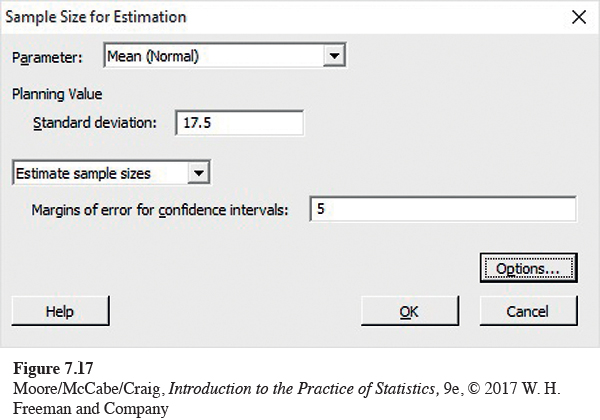
Figure 7.17 shows the Minitab input window used to do these calculations. Because the default confidence level is 95%, only the desired margin of error m and the estimate for s need to be entered.

463

Figure 7.17: FIGURE 7.17 Minitab input window used to compute the sample size for the desired margin of error, Example 7.21.

Note that the n = 50 refers to the expected margin of error being no more than five hours. This does not guarantee that the margin of error for the collected sample will be less than five hours. That is because the sample standard deviation s varies sample to sample and these calculations are treating it as a fixed quantity. More advanced sample size procedures ask you to also specify the probability of obtaining a margin of error less than the desired value. For our approach, this probability is roughly 50%. For a probability closer to 100%, the sample size will need to be larger. For example, suppose we wanted this probability to be roughly 80%. In SAS, we’d perform these calculations using the command

proc power;

onesamplemeans CI=t stddev=17.5 halfwidth=5 probwidth=0.80 ntotal=.;

run;

The needed sample size increases from n = 50 to n = 57.

Unfortunately, the actual number of usable observations is often less than that planned at the beginning of a study. This is particularly true of data collected in surveys or studies that involve a time commitment from the participants. Careful study designers often assume a nonresponse rate or dropout rate that specifies what proportion of the originally planned sample will fail to provide data. We use this information to calculate the sample size to be used at the start of the study. For example, if, in the preceding survey, we expect only 40% of those students to respond, we would need to start with a sample size of 2.5 × 50 =125 to obtain usable information from 50 students.

nonresponse, p. 196

These sample size calculations also do not account for collection costs. In practice, taking observations costs time and money. There are times when the required sample size may be impossibly expensive. In those situations, one might consider a larger margin of error and/or a lower confidence level to be acceptable.

For the two-sample t confidence interval, the margin of error is

A similar type of iterative search can be used to determine the sample sizes n₁ and n₂, but now we need to guess both standard deviations and decide on an estimate for the degrees of freedom. We suggest taking the conservative approach and using the smaller of n₁ − 1 and n₂ − 1 for the degrees of freedom. Another approach is to consider the standard deviations and sample sizes are equal, so the margin of error is

and use degrees of freedom 2(n − 1). That is the approach most statistical software take.

464

EXAMPLE 7.22

Planning a new blood pressure study. In Example 7.20 (page 452), we calculated a 90% confidence interval for the mean difference in blood pressure. The 90% margin of error was roughly 5.6 mm Hg. Suppose that a new study is being planned and the desired margin of error at 90% confidence is 2.8 mm Hg. How many subjects per group do we need?

The pooled sample standard deviation in Example 7.20 is 7.385. To be a bit conservative, we’ll guess that the two population standard deviations are both 8.0. To compute an initial n, we replace t* with z*. This results in

We round up to get n = 45. The following table summarizes the margin of error for this and some larger values of n.

n
45	2.834
46	2.801
47	2.770

The requirement is first satisfied when n = 47. In SAS, we’d perform these calculations using the command

proc power;

twosamplemeans CI=diff alpha=0.1 stddev=8 halfwidth=2.8

probwidth=0.50 npergroup=.;

run;

This sample size is roughly 4.5 times the sample size used in Example 7.20. This researcher may not be able to recruit this large a sample. If so, we should consider a larger margin of error.

USE YOUR KNOWLEDGE

Question 7.93

7.93 Starting salaries. In a recent survey by the National Association of Colleges and Employers, the average starting salary for college graduate with a computer and information sciences degree was reported to be $62,194.⁴⁰ You are planning to do a survey of starting salaries for recent computer science majors from your university. Using an estimated standard deviation of $11,605, what sample size do you need to have a margin of error equal to $5000 with 95% confidence?

465

Question 7.94

7.94 Changes in sample size. Suppose that, in the setting of the previous exercise, you have the resources to contact 35 recent graduates. If all respond, will your margin of error be larger or smaller than $5000? What if only 50% respond? Verify your answers by performing the calculations.

The power of the one-sample t test The power of a statistical test measures its ability to detect deviations from the null hypothesis. In practice, we carry out the test in the hope of showing that the null hypothesis is false, so high power is important. Power calculations are a way to assess whether or not a sample size is sufficiently large to answer the research question.

The power of the one-sample t test against a specific alternative value of the population mean μ is the probability that the test will reject the null hypothesis when this alternative is true. To calculate the power, we assume a fixed level of significance, usually α = 0.05.

Calculation of the exact power of the t test takes into account the estimation of σ by s and requires a new distribution. We will describe that calculation when discussing the power of the two-sample t test. Fortunately, an approximate calculation that is based on assuming that σ is known is almost always adequate for planning a study in the one-sample case. This calculation is very much like that for the z test, presented in Section 6.4. The steps are

power calculation, p. 392

1. Write the event, in terms of , that the test rejects H₀.
2. Find the probability of this event when the population mean has the alternative value.

Here is an example.

EXAMPLE 7.23

Is the sample size large enough? Recall Example 7.2 (page 413) on the average time that U.S. college students spend watching traditional television. The sample mean of n = 8 students was four hours lower than the U.S. average of 18- to 24-year-olds but not found significantly different. Suppose a new study is being planned using a sample size of n = 50 students. Does this study have adequate power when the population mean is four hours less than the U.S. average?

We wish to compute the power of the t test for

H₀: μ = 18.5

H_a: μ < 18.5

against the alternative that μ = 18.5 − 4 = 14.5 when n = 50. This gives us most of the information we need to compute the power. The other important piece is a rough guess of the size of σ. In planning a large study, a pilot study is often run for this and other purposes. In this case, we can use the standard deviation from the earlier survey. Similar to Example 7.21, we will round up and use σ = 17.5 and s = 17.5 in the approximate calculation.

Step 1. The t test with 50 observations rejects H₀ at the 5% significance level if the t statistic

is less than the lower 5% point of t(49), which is −1.677. Taking s = 17.5, the event that the test rejects H₀ is, therefore,

466

Step 2. The power is the probability that when μ = 14.5. Taking σ = 17.5, we find this probability by standardizing :

= P(Z ≤ −0.061)

= 0.4761

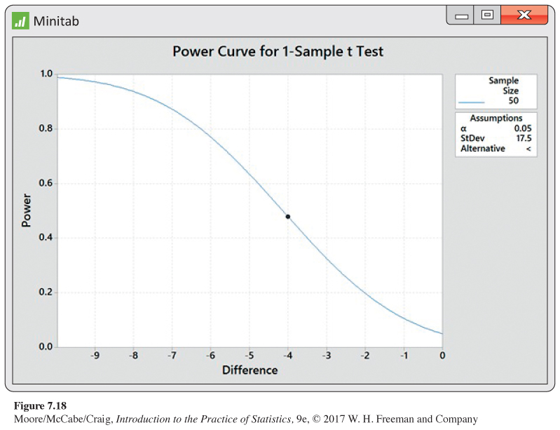
A mean value of 14.5 hours per week will produce significance at the 5% level in only 47.6% of all possible samples. Figure 7.18 shows Minitab output for the exact power calculation. It is about 48% and is represented by a dot on the power curve at a difference of −4. This curve is very informative. For many studies, 80% is considered the standard value for desirable power. We see that with a sample size of 50, the power is greater than 80% only for reductions larger than 6.25 hours per week. If we want to detect a reduction of only four hours, we definitely need to increase the sample size.

Figure 7.18: FIGURE 7.18 Minitab output (a power curve) for the one-sample power calculation, Example 7.23.

467

Power calculations are used in planning studies to ensure that we have a reasonable chance of detecting effects of interest. They give us some guidance in selecting a sample size. In making these calculations, we need assumptions about the standard deviation and the alternative of interest. In our example, we assumed that the standard deviation would be 17.5, but in practice, we are hoping that the value will be somewhere around this value. Similarly, we have used a somewhat arbitrary alternative of 14.5. This is a guess based on the results of the previous study. Beware of putting too much trust in fine details of the results of these calculations. They serve as a guide, not a mandate.

USE YOUR KNOWLEDGE

Question 7.95

7.95 Power for other values of μ. If you repeat the calculation in Example 7.23 for values of μ that are smaller than 14.5, would you expect the power to be higher or lower than 0.4761? Why?

Question 7.96

7.96 Another power calculation. Verify your answer to the previous exercise by doing the calculation for the alternative μ = 12 hours per week.

The power of the two-sample t test The two-sample t test is one of the most used statistical procedures. Unfortunately, because of inadequate planning, users frequently fail to find evidence for the effects that they believe to be present. This is often the result of an inadequate sample size. Power calculations, performed prior to running the experiment, will help avoid this occurrence.

We just learned how to approximate the power of the one-sample t test. The basic idea is the same for the two-sample case, but we will describe the exact method rather than an approximation again. The exact power calculation involves a new distribution, the noncentral t distributionnoncentral t distribution. This calculation is not practical by hand but is easy with software that calculates probabilities for this distribution.

We consider only the common case where the null hypothesis is “no difference,’’ μ₁ −μ₂ = 0. We illustrate the calculation for the pooled two-sample t test. A simple modification is needed when we do not pool. The unknown parameters in the pooled t setting are μ₁, μ₂, and a single common standard deviation σ. To find the power for the pooled two-sample t test, follow these steps.

Step 1. Specify these quantities:

(a) An alternative value for μ₁ −μ₂ that you consider important to detect.
(b) The sample sizes, n₁ and n₂.
(c) A fixed significance level α, often α = 0.05.
(d) An estimate of the standard deviation σ from a pilot study or previous studies under similar conditions.

Step 2. Find the degrees of freedom df = n₁ + n₂ − 2 and the value of t* that will lead to rejecting H₀ at your chosen level α.

468

Step 3. Calculate the noncentrality parameternoncentrality parameter

Step 4. The power is the probability that a noncentral t random variable with degrees of freedom df and noncentrality parameter δ will be greater than t*. Use software to calculate this probability. In SAS, the command is 1 - PROBT(tstar, df, delta). In R the commmand is 1-pt(tstar, df, delta). If you do not have software that can perform this calculation, you can approximate the power as the probability that a standard Normal random variable is greater than t* −δ, that is, P(Z > t* −δ). Use Table A or software for standard Normal probabilities.

Note that the denominator in the noncentrality parameter,

is our guess at the standard error for the difference in the sample means. Therefore, if we wanted to assess a possible study in terms of the margin of error for the estimated difference, we would examine t* times this quantity.

If we do not assume that the standard deviations are equal, we need to guess both standard deviations and then combine these to get an estimate of the standard error:

This guess is then used in the denominator of the noncentrality parameter. Use the conservative value, the smaller of n₁ − 1 and n₂ − 1, for the degrees of freedom.

EXAMPLE 7.24

Planning a new study of calcium versus placebo groups. In Example 7.19 (page 451), we examined the effect of calcium on blood pressure by comparing the means of a treatment group and a placebo group using a pooled two-sample t test. The P-value was 0.059, failing to achieve the usual standard of 0.05 for statistical significance. Suppose that we wanted to plan a new study that would provide convincing evidence—say, at the 0.01 level—with high probability. Let’s examine a study design with 45 subjects in each group (n₁ = n₂ = 45) to see if this meets our goals.

Step 1. Based on our previous results, we choose μ₁ −μ₂ = 5 as an alternative that we would like to be able to detect with α = 0.01. For σ we use 7.4, our pooled estimate from Example 7.19.

Step 2. The degrees of freedom are n₁ + n₂ − 2 = 88, which leads to t* = 2.37 for the significance test.

Step 3. The noncentrality parameter is

469

Step 4. Software gives the power as 0.7965, or 80%. The Normal approximation gives 0.7983, a very accurate result.

With this choice of sample sizes, we are just barely below 80% power. If we judge this to be large enough power, we can proceed to the recruitment of our samples.

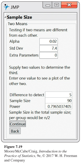
With software it is often very easy to examine the effects of variations in a study design. For example, Figure 7.19 shows the JMP power calculator for the two-sample t test. You input values for α, σ, n₁ + n₂, and δ (Step 1) and it computes the power (Steps 2–4). Figure 7.19 shows the results of the calculations for Example 7.24. The JMP calculator only considers the two-sided alternative so to get the power for a one-sided alternative, the significance level must be input as 2α. Most other software, such as Minitab, provides the option to choose the alternative.

USE YOUR KNOWLEDGE

Question 7.97

7.97 Power and the choice of alternative. If you were to repeat the calculation in Example 7.24 for the two-sided alternative, would the power increase or decrease? Explain your answer.

Question 7.98

7.98 Power and the standard deviation. If the true population standard deviation were 8 instead of the 7.4 hypothesized in Example 7.24, would the power increase or decrease? Explain.

Question 7.99

7.99 Power and statistical software. Refer to the two previous exercises. Use statistical software to compute the exact power of each scenario.

Figure 7.19: FIGURE 7.19 JMP input/output window for the two-sample power calculation, Example 7.24.

470

Inference for non-Normal populations

We have not discussed how to do inference about the mean of a clearly non-Normal distribution based on a small sample. If you face this problem, you should consult an expert. Three general strategies are available:

• In some cases, a distribution other than a Normal distribution describes the data well. There are many non-Normal models for data, and inference procedures for these models are available.
• Because skewness is the chief barrier to the use of t procedures on data without outliers, you can attempt to transform skewed data so that the distribution is symmetric and as close to Normal as possible. Confidence levels and P-values from the t procedures applied to the transformed data will be quite accurate for even moderate sample sizes. Methods are generally available for transforming the results back to the original scale.
• Use a distribution-freedistribution-free procedures inference procedure. Such procedures do not assume that the population distribution has any specific form, such as Normal. Distribution-free procedures are often called nonparametric proceduresnonparametric procedures. Chapter 15 discusses several of these procedures.

Each of these strategies can be effective, but each quickly carries us beyond the basic practice of statistics. We emphasize procedures based on Normal distributions because they are the most common in practice, because their robustness makes them widely useful, and (most important) because we are first of all concerned with understanding the principles of inference. Therefore, we will not discuss procedures for non-Normal continuous distributions. We will be content with illustrating by example the use of a transformation and of a simple distribution-free procedure.

log transformation, p. 91

Transforming data When the distribution of a variable is skewed, it often happens that a simple transformation results in a variable whose distribution is symmetric and even close to Normal. The most common transformation is the logarithm, or log. The logarithm tends to pull in the right tail of a distribution. For example, the data 2, 3, 4, 20 show an outlier in the right tail. Their common logarithms 0.30, 0.48, 0.60, 1.30 are much less skewed. Taking logarithms is a possible remedy for right-skewness. Instead of analyzing values of the original variable X, we compute their logarithms and analyze the values of log X. Here is an example of this approach.

EXAMPLE 7.25

Justin Sullivan/Staff/Getty Images

Length of audio files on an iPod. Table 7.5 presents data on the length (in seconds) of audio files found on an iPod. There was a total of 10,003 audio files, and 50 files were randomly selected using the “shuffle songs’’ command.⁴¹ We would like to give a confidence interval for the average audio file length μ for this iPod.

Table : TABLE 7.5 Length (in Seconds) of Audio Files Sampled from an iPod

240	316	259	46	871	411	1366
233	520	239	259	535	213	492
315	696	181	357	130	373	245
305	188	398	140	252	331	47
309	245	69	293	160	245	184
326	612	474	171	498	484	271
207	169	171	180	269	297	266
1847

471

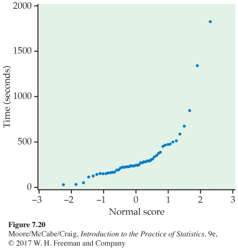
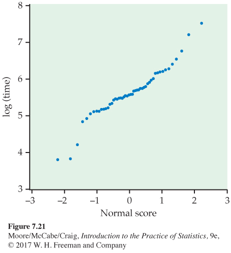
Figure 7.20: FIGURE 7.20 Normal quantile plot of audio file length, Example 7.25. This sort of pattern occurs when a distribution is skewed to the right.

Figure 7.21: FIGURE 7.21 Normal quantile plot of the logarithms of the audio file lengths, Example 7.25. This distribution appears approximately Normal.

A Normal quantile plot of the audio data from Table 7.5 (Figure 7.20) shows that the distribution is skewed to the right. Because there are no extreme outliers, the sample mean of the 50 observations will nonetheless have an approximately Normal sampling distribution. The t procedures could be used for approximate inference. For more exact inference, we will transform the data so that the distribution is more nearly Normal. Figure 7.21 is a Normal quantile plot of the natural logarithms of the time measurements. The transformed data are very close to Normal, so t procedures will give quite exact results.

The application of the t procedures to the transformed data is straightforward. Call the original length values from Table 7.5 the variable X. The transformed data are values of . In most software packages, it is an easy task to transform data in this way and then analyze the new variable.

EXAMPLE 7.26

Software output of audio length data. Analysis of the natural log of the length values in Minitab produces the following output:

N	Mean	StDev	SE Mean	95.0% C.I.
50	5.6315	0.6840	0.0967	(5.4371, 5.8259)

For comparison, the 95% t confidence interval for the original mean μ is found from the original data as follows:

N	Mean	StDev	SE Mean	95.0% C.I.
50	354.1	307.9	43.6	(266.6, 441.6)

472

The advantage of analyzing transformed data is that use of procedures based on the Normal distributions is better justified and the results are more exact. The disadvantage is that a confidence interval for the mean μ in the original scale (in our example, seconds) cannot be easily recovered from the confidence interval for the mean of the logs. One approach based on the lognormal distribution⁴² results in an interval of (285.5, 435.5), which is narrower and slightly asymmetric compared with the t interval.

Use of a distribution-free procedure Perhaps the most straightforward way to cope with non-Normal data is to use a distribution-free, or nonparametric, procedure. As the name indicates, these procedures do not require the population distribution to have any specific form, such as Normal. Distribution-free significance tests are quite simple and are available in most statistical software packages.

Distribution-free tests have two drawbacks. First, they are generally less powerful than tests designed for use with a specific distribution, such as the t test. Second, we must often modify the statement of the hypotheses in order to use a distribution-free test. A distribution-free test concerning the center of a distribution, for example, is usually stated in terms of the median rather than the mean. This is sensible when the distribution may be skewed. But the distribution-free test does not ask the same question (Has the mean changed?) that the t test does.

The simplest distribution-free test, and one of the most useful, is the sign testsign test. The test gets its name from the fact that we look only at the signs of the differences, not their actual values. The following example illustrates this test.

EXAMPLE 7.27

The effect of altering a software parameter. Example 7.7 (page 419) describes an experiment to compare the measurements obtained from two software algorithms. In that example, we used the matched pairs t test on these data, despite some skewness, which makes the P-value only roughly correct. The sign test is based on the following simple observation: of the 51 parts measured, 29 had a larger measurement with the option off and 22 had a larger measurement with the option on.

To perform a significance test based on these counts, let p be the probability that a randomly chosen part would have a larger measurement with the option turned on. The null hypothesis of “no effect’’ says that these two measurements are just repeat measurements, so the measurement with the option off is equally likely to be larger or smaller than the measurement with the option on. Therefore, we want to test

H₀: p = 1/2

H_a: p ≠ 1/2

binomial distribution, p. 312

The 51 parts are independent trials, so the number that had larger measurements with the option off has the binomial distribution B(51, 1/2) if H₀ is true. The P-value for the observed count 29 is, therefore, 2P(X ≥ 29), where X has the B(51, 1/2) distribution. You can compute this probability with software or the Normal approximation to the binomial:

= 2P (Z ≥ 0.98)

= 2(0.1635)

= 0.3270

473

As in Example 7.7, there is not strong evidence that the two measurements are different.

There are several varieties of sign test, all based on counts and the binomial distribution. The sign test for matched pairs is the most useful. The null hypothesis of “no effect’’ is then always H₀: p = 1/2. The alternative can be one-sided in either direction or two-sided, depending on the type of change we are considering.

SIGN TEST FOR MATCHED PAIRS

Ignore pairs with difference 0; the number of trials n is the count of the remaining pairs. The test statistic is the count X of pairs with a positive difference. P-values for X are based on the binomial B(n, 1/2) distribution.

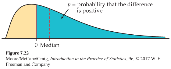
The matched pairs t test in Example 7.7 tested the hypothesis that the mean of the distribution of differences is 0. The sign test in Example 7.27 is, in fact, testing the hypothesis that the median of the differences is 0. If p is the probability that a difference is positive, then p = 1/2 when the median is 0. This is true because the median of the distribution is the point with probability 1/2 lying to its right. As Figure 7.22 illustrates, p > 1/2 when the median is greater than 0, again because the probability to the right of the median is always 1/2. The sign test of H₀: p =1/2 against H_a: p > 1/2 is a test of

H₀: population median = 0

H_a: population median > 0

The sign test in Example 7.27 makes no use of the actual scores—it just counts how many parts had a larger measurement with the option off. Any parts that did not have different measurements would be ignored altogether. Because the sign test uses so little of the available information, it is much less powerful than the t test when the population is close to Normal. Chapter 15 describes other distribution-free tests that are more powerful than the sign test.

USE YOUR KNOWLEDGE

Question 7.100

7.100 Sign test for the oil-free frying comparison. Exercise 7.10 (page 422) gives data on the taste of hash browns made using a hot-oil fryer and an oil-free fryer. Is there evidence that the medians are different? State the hypotheses, carry out the sign test, and report your conclusion.

Figure 7.22: FIGURE 7.22 Why the sign test tests the median difference: when the median is greater than 0, the probability p of a positive difference is greater than 1/2, and vice versa.