8.2 8.2 Comparing Two Proportions
505
When you complete this section, you will be able to:
• Identify the counts and sample sizes for a comparison between two proportions, compute the sample proportions, and find their difference.
• Apply the guidelines for when to use the large-sample confidence interval for a difference between two proportions.
• Apply the large-sample method to find the confidence interval for a difference between two proportions and interpret the confidence interval.
• Apply the guidelines for when to use the large-sample significance test for a difference between two proportions.
• Apply the large-sample method to perform a significance test for comparing two proportions and interpret the results of the significance test.
• Find the sample size needed for a desired margin of error for the difference in proportions.
• Find the sample size needed for a significance test for comparing two proportions.
• Calculate and interpret the relative risk.
Because comparative studies are so common, we often want to compare the proportions of two groups (such as men and women) that have some characteristic. In the previous section, we learned how to estimate a single proportion. Our problem now concerns the comparison of two proportions.
We call the two groups being compared Population 1 and Population 2 and the two population proportions of “successes” p1 and p2. The data consist of two independent SRSs, of size n1 from Population 1 and size n2 from Population 2. The proportion of successes in each sample estimates the corresponding population proportion. Here is the notation we will use in this section:
| Population | Sample | Count of | Sample | |
|---|---|---|---|---|
| Population | proportion | size | successes | proportion |
| 1 | p1 | n1 | X1 | |
| 2 | p2 | n2 | X2 |
To compare the two populations, we use the difference between the two sample proportions:
When both sample sizes are sufficiently large, the sampling distribution of the difference D is approximately Normal.
Inference procedures for comparing proportions are z procedures based on the Normal approximation and on standardizing the difference D. The first step is to obtain the mean and standard deviation of D. By the addition rule for means, the mean of D is the difference of the means:
506
addition rule for means, p. 254
addition rule for variances, p. 258
That is, the difference between the sample proportions is an unbiased estimator of the population difference p1 − p2. Similarly, the addition rule for variances tells us that the variance of D is the sum of the variances:
Therefore, when n1 and n2 are large, D is approximately Normal with mean μD = p1 − p2 and standard deviation
USE YOUR KNOWLEDGE
Question 8.47
8.47 Rules for means and variances. Suppose that p1 = 0.4, n1 = 25, p2 = 0.5, n2 = 30. Find the mean and the standard deviation of the sampling distribution of p1 − p2.
Question 8.48
8.48 Effect of the sample sizes. Suppose that p1 = 0.4, n1 = 100, p2 = 0.5, n2 = 120.
(a) Find the mean and the standard deviation of the sampling distribution of p1 − p2.
(b) The sample sizes here are four times as large as those in the previous exercise while the population proportions are the same. Compare the results for this exercise with those that you found in the previous exercise. What is the effect of multiplying the sample sizes by 4?
Question 8.49
8.49 Rules for means and variances. It is quite easy to verify the formulasfor the mean and standard deviation of the difference D.
(a) What are the means and standard deviations of the two sample proportions and ?
(b) Use the addition rule for means of random variables: what is the mean of ?
(c) The two samples are independent. Use the addition rule for variances of random variables: what is the variance of D?
Large-sample confidence interval for a difference in proportions
To obtain a confidence interval for p1 − p2, we once again replace the unknown parameters in the standard deviation with estimates to obtain an estimated standard deviation, or standard error. Here is the confidence interval we want.
507
LARGE-SAMPLE CONFIDENCE INTERVAL FOR COMPARING TWO PROPORTIONS
Choose an SRS of size n1 from a large population having proportion p1 of successes and an independent SRS of size n2 from another population having proportion p2 of successes. The estimate of the difference in the population proportions is
The standard error of D is
and the margin of error for confidence level C is
where the critical value z* is the value for the standard Normal density curve with area C between −z* and z*. An approximate level C confidence interval for p1 − p2 is
D ± m
Use this method for 90%, 95%, or 99% confidence when the number of successes and the number of failures in each sample are both 10 or more.
EXAMPLE 8.11
Who uses Instagram? A recent study compared the proportions of young women and men who use Instagram.15 A total of 1069 young women and men were surveyed. These are the cases for the study. The response variable is User with values Yes and No. The explanatory variable is Sex with values “Men” and “Women.” Here are the data:
| Sex | n | X | |
|---|---|---|---|
| Women | 537 | 328 | 0.6108 |
| Men | 532 | 234 | 0.4398 |
| Total | 1069 | 562 | 0.5257 |
In this table, the column gives the sample proportions of women and men who use Instagram. The proportion for the total sample is given in the last entry in this column.
Let’s find a 95% confidence interval for the difference between the proportions of women and of men who use Instagram. We first find the difference in the proportions:
= 0.6108 − 0.4398
= 0.1710
508
Then we calculate the standard error of D:
= 0.0301
For 95% confidence, we have z* = 1.96, so the margin of error is
The 95% confidence interval is
D ± m = 0.1710 ± 0.0590
= (0.112, 0.230)
With 95% confidence, we can say that the difference in the proportions is between 0.112 and 0.230. Alternatively, we can report that the difference between the percent of women who are Instagram users and the percent of men who are Instagram users is 17.1%, with a 95% margin of error of 5.9%.
In this example, men and women were not sampled separately. The sample sizes are, in fact, random and reflect the gender distributions of the subjects who responded to the survey. Two-sample significance tests and confidence intervals are still approximately correct in this situation.
In the preceding example, we chose women to be the first population. Had we chosen men to be the first population, the estimate of the difference would be negative (−0.1710). Because it is easier to discuss positive numbers, we generally choose the first population to be the one with the higher proportion.
EXAMPLE 8.12
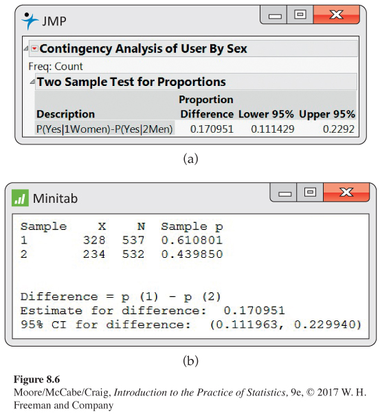
Instagram confidence interval from software. Figure 8.5 shows a spreadsheet that can be used as input to software. Output from JMP and Minitab is given in Figure 8.6. Compare these outputs with the calculations that we performed in Example 8.11.

509
USE YOUR KNOWLEDGE
Question 8.50
8.50 Gender and commercial preference. A study was designed to compare two energy drink commercials. Each participant was shown the commercials in random order and asked to select the better one. Commercial A was selected by 54 out of 115 women and 83 out of 145 men. Give an estimate of the difference in gender proportions that favored Commercial A. Also construct a large-sample 95% confidence interval for this difference.
Question 8.51
8.51 Gender and commercial preference, revisited. Refer to Exercise 8.50. Construct a 95% confidence interval for the difference in proportions that favor Commercial B. Explain how you could have obtained these results from the calculations you did in Exercise 8.50.
BEYOND THE BASICS
The Plus Four Confidence Interval for a Difference in Proportions
Just as in the case of estimating a single proportion, a small modification of the sample proportions can greatly improve the accuracy of confidence intervals.16 As before, we add two successes and two failures to the actual data, but now we divide them equally between the two samples. That is, we add one success and one failure to each sample. This method can be used for 90%, 95%, or 99% confidence when both sample sizes are at least five. Here is an example.
510
EXAMPLE 8.13
Gender and sexual maturity. In studies that look for a difference between genders, a major concern is whether or not apparent differences are due to other variables that are associated with gender. Because boys mature more slowly than girls, a study of adolescents that compares boys and girls of the same age may confuse a gender effect with an effect of sexual maturity. The “Tanner score” is a commonly used measure of sexual maturity.17 Subjects are asked to determine their score by placing a mark next to a rough drawing of an individual at their level of sexual maturity. There are five different drawings, so the score is an integer between 1 and 5.
A pilot study included 12 girls and 12 boys from a population that will be used for a large experiment. Four of the boys and three of the girls had Tanner scores of 4 or 5, a high level of sexual maturity. Let’s find a 95% confidence interval for the difference between the proportions of boys and girls who have high (4 or 5) Tanner scores in this population. The numbers of successes and failures in both groups are not all at least 10, so the large-sample approach is not recommended. On the other hand, the sample sizes are both at least 5, so the plus four method is appropriate.
The plus four estimate of the population proportion for boys is
For girls, the estimate is
Therefore, the estimate of the difference is
The standard error of is
= 0.1760
For 95% confidence, z* = 1.96 and the margin of error is
The confidence interval is
= (−0.274, 0.416)
With 95% confidence, we can say that the difference in the proportions is between −0.274 and 0.416. Alternatively, we can report that the difference in the proportions of boys and girls with high Tanner scores in this population is 7.1% with a 95% margin of error of 34.5%.
511
![]()
The very large margin of error in this example indicates that either boys or girls could be more sexually mature in this population and that the difference could be quite large. Although the interval includes the possibility that there is no difference, corresponding to p1 = p2 or p1 − p2 = 0, we should not conclude that there is no difference in the proportions. With small sample sizes such as these, the data do not provide us with a lot of information for our inference. This fact is expressed quantitatively through the very large margin of error.
Significance test for a difference in proportions
Although we prefer to compare two proportions by giving a confidence interval for the difference between the two population proportions, it is sometimes useful to test the null hypothesis that the two population proportions are the same.
We standardize by subtracting its mean p1 − p2 and then dividing by its standard deviation
If n1 and n2 are large, the standardized difference is approximately N(0, 1). For the large-sample confidence interval we used sample estimates in place of the unknown population values in the expression for σD. Although this approach would lead to a valid significance test, we instead adopt the more common practice of replacing the unknown σD with an estimate that takes into account our null hypothesis H0: p1 = p2. If these two proportions are equal, then we can view all the data as coming from a single population. Let p denote the common value of p1 and p2; then the standard deviation of is
We estimate the common value of p by the overall proportion of successes in the two samples:
This estimate of p is called the pooled estimatepooled estimate of p because it combines, or pools, the information from both samples.
To estimate σD under the null hypothesis, we substitute for p in the expression for σD. The result is a standard error for D that assumes H0: p1 = p2:
The subscript on SEDp reminds us that we pooled data from the two samples to construct the estimate.
512
SIGNIFICANCE TEST FOR COMPARING TWO PROPORTIONS
To test the hypothesis
H0: p1 = p2
compute the z statistic
where the pooled standard error is
and where the pooled estimate of the common value of p1 and p2 is
In terms of a standard Normal random variable Z, the approximate P-value for a test of H0 against
Ha: p1 > p2 is P(Z ≥ z) 
Ha: p1 < p2 is P(Z ≤ z) 
Ha: p1 ≠ p2 is 2P(Z ≥ |z|) 
This z test is based on the Normal approximation to the binomial distribution. As a general rule, we will use it when the number of successes and the number of failures in each of the samples are at least 5.
EXAMPLE 8.14
Sex and Instagram use: The z test. Are young women and men equally likely to say they use Instagram? We examine the data in Example 8.11 (page 507) to answer this question. Here is the data summary:
| Sex | n | X | |
|---|---|---|---|
| Women | 537 | 328 | 0.6108 |
| Men | 532 | 234 | 0.4398 |
| Total | 1069 | 562 | 0.5257 |
The sample proportions are certainly quite different, but we will perform a significance test to see if the difference is large enough to lead us to believe that the population proportions are not equal. Formally, we test the hypotheses
H0: p1 = p2
Ha: p1 ≠ p2
513
The pooled estimate of the common value of p is
Note that this is the estimate on the bottom line of the preceding data summary. The test statistic is calculated as follows:
= 5.60
The P-value is 2P(Z ≥ 5.60). Note that the largest value for z in Table A is 3.49. Therefore, from Table A, we can conclude that P < 2(1 − 0.9998) = 0.0004, although we know that the true P value is smaller.
Here is our summary: 61% of the women and 44% of the men are Instagram users; the difference is statistically significant (z = 5.60, P < 0.0004).
EXAMPLE 8.15
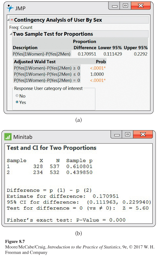
Output for the Instagram significance test. We prefer to use software to obtain the significance test results for comparing the Instagram use of young women and men. Output from JMP and Minitab is given in Figure 8.7. JMP reports the significance tests for the two-sided alternative and for the two one-sided alternatives. We are interested in the two-sided alternative.
514
Therefore, we report the P-value as < 0.0001. Minitab reports the test statistic, z = 5.60, and gives the P-value as 0.000 (this means P < 0.0005) for the Fisher exact test. This test is an alternative to the large-sample significance test that we have discussed. It is preferred by many, particularly for small sample sizes.
Do you think that we could have argued that the proportion would be higher for women than for men before looking at the data in this example? This would allow us to use the one-sided alternative Ha: p1 > p2. The P-value would be half of the value obtained for the two-sided test. Do you think that this approach is justified?
USE YOUR KNOWLEDGE
Question 8.52
8.52 Gender and commercial preference: the z test. Refer to Exercise 8.50 (page 509). Test whether the proportions of women and men who liked Commercial A are the same versus the two-sided alternative at the 5% level.
Question 8.53
8.53 Changing the alternative hypothesis. Refer to the previous exercise. Does your conclusion change if you test whether the proportion of men who favor Commercial A is larger than the proportion of females? Explain.
Choosing a sample size for two sample proportions
In Section 8.1, we studied methods for determining the sample size using two settings. First, we used the margin of error for a confidence interval for a single proportion as the criterion for choosing n (page 495). Second, we used the power of the significance test for a single proportion as the determining factor (page 498). We follow the same approach here for comparing two proportions.
Use the margin of error Recall that the large-sample estimate of the difference in proportions is
the standard error of the difference is
and the margin of error for confidence level C is
m = z*SED
where z* is the value for the standard Normal density curve with area C between −z* and z*.
515
For a single proportion, we guessed a value for the true proportion and computed the margins of error for various choices of n. Here, we use the same idea but we need to guess values for the two proportions. We can display the results in a table, as in Example 8.9 (page 497), or in a graph, as in Exercise 8.43 (page 504).
SAMPLE SIZE FOR DESIRED MARGIN OF ERROR
The level C confidence interval for a difference in two proportions will have a margin of error approximately equal to a specified value m when the sample size for each of the two proportions is
Here, z* is the critical value for confidence C, and and are guessed values for p1 and p2, the proportions of successes in the future sample.
The margin of error will be less than or equal to m if and are chosen to be 0.5. The common sample size required is then given by
Note that to use the confidence interval, which is based on the Normal approximation, we still require that the number of successes and the number of failures in each of the samples are at least 10.
EXAMPLE 8.16
Confidence interval–based sample sizes for preferences of women and men. Consider the setting in Exercise 8.50, where we compared the preferences of women and men for two commercials. Suppose we want to do a study in which we perform a similar comparison using a 95% confidence interval that will have a margin of error of 0.1 or less. What should we choose for our sample size? Using m = 0.1 and z* in our formula, we have
We would include 192 women and 192 men in our study.
516
Note that we have rounded the calculated value, 192.08, down because it is very close to 192. The normal procedure would be to round the calculated value up to the next larger integer.
USE YOUR KNOWLEDGE
Question 8.54
8.54 What would the margin of error be? Consider the setting in Exercise 8.50.
(a) Compute the margins of error for n1 = 24 and n2 = 24 for each of the following scenarios: p1 = 0.6, p2 = 0.5; p1 = 0.7, p2 = 0.5; and p1 = 0.8, p2 = 0.5.
(b) If you think that any of these scenarios is likely to fit your study, should you reconsider your choice of n1 = 24 and n2 = 24? Explain your answer.
Use the power of the significance test When we studied using power to compute the sample size needed for a significance test for a single proportion, we used software. We will do the same for the significance test for comparing two proportions.
Some software allows us to consider significance tests that are a little more general than the version we studied in this section. Specifically, we used the null hypothesis H0: p1 = p2, which we can rewrite as H0: p1 − p2 = 0. The generalization allows us to use values different from zero in the alternative way of writing H0. Therefore, we write H0: p1 − p2 = Δ0 for the null hypothesis, and we will need to specify Δ0 = 0 for the significance test that we studied.
Here is a summary of the inputs needed for software to perform the calculations:
• The value of Δ0 in the null hypothesis H0: p1 − p2 = Δ0.
• The alternative hypothesis, two-sided (Ha: p1 ≠ p2) or one-sided (Ha: p1 > p2 or Ha: p1 < p2).
• Values for p1 and p2 in the alternative hypothesis.
• The Type I error (α, the probability of rejecting the null hypothesis when it is true); usually we choose 5% (α = 0.05) for the Type I error.
• Power (probability of rejecting the null hypothesis when it is false); usually we choose 80% (0.80) for power.
EXAMPLE 8.17
Sample sizes for preferences of women and men. Refer to Example 8.16 where we used the margin of error to find the sample sizes for comparing the preferences of women and men for two commercials. Let’s find the sample sizes required for a significance test that the two proportions who prefer Commercial A are equal (Δ0 = 0) using a two-sided alternative with p1 = 0.6 and p2 = 0.4, α = 0.05, and 80% (0.80) power. Outputs from JMP and Minitab are given in Figure 8.8. We need n1 = 97 women and n2 = 97 men for our study.
517
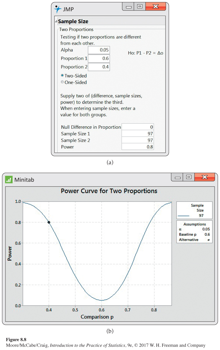
Note that the Minitab output [Figure 8.8(b)] gives the power curve for different alternatives. All of these have p1 = 0.6, which Minitab calls the “Comparison p,” while p2 varies from 0.3 to 0.9. We see that the power is essentially 100% (1) at these extremes. It is 0.05, the type I error, at p2 = 0.6, which corresponds to the null hypothesis.
518
USE YOUR KNOWLEDGE
Question 8.55
8.55 Find the sample sizes. Consider the setting in Example 8.17. Change p1 to 0.85 and p2 to 0.90. Find the required sample sizes.
BEYOND THE BASICS
Relative Risk
We compared Instagram use for women and men by reporting the difference in the proportions with a confidence interval. Another way to compare two proportions is to take the ratio. This approach can be used in any setting and it is particularly common in medical settings.
We think of each proportion as a riskrisk that something (usually bad) will happen. We then compare these two risks with the ratio of the two proportions, which is called the relative riskrelative risk (RR). Note that a relative risk of 1 means that the two proportions, and , are equal. The procedure for calculating confidence intervals for relative risk is based on the same kind of principles that we have studied, but the details are somewhat more complicated. Fortunately, we can leave the details to software and concentrate on interpretation and communication of the results.
EXAMPLE 8.18
Aspirin and blood clots: Relative risk. A study of patients who had blood clots (venous thromboembolism) and had completed the standard treatment were randomly assigned to receive a low-dose aspirin or a placebo treatment. The 822 patients in the study were randomized to the treatments, 411 to each. Patients were monitored for several years for the occurrence of several related medical conditions. Counts of patients who experienced one or more of these conditions were reported for each year after the study began.18 The following table gives the data for a composite of events, termed “major vascular events.” Here, X is the number of patients who had a major event.
| Population | n | X | |
|---|---|---|---|
| 1 (aspirin) | 411 | 45 | 0.1095 |
| 2 (placebo) | 411 | 73 | 0.1776 |
| Total | 822 | 118 | 0.1436 |
The relative risk is
Software gives the 95% confidence interval as 0.4364 to 0.8707. Taking aspirin has reduced the occurrence of major events to 62% of what it is for patients taking the placebo. The 95% confidence interval is 44% to 87%.
Note that the confidence interval is not symmetric about the estimate. Relative risk is one of many situations where this occurs.