9.2 9.2 Goodness of Fit
When you complete this section, you will be able to:
• Compute expected counts given a sample size and the probabilities specified by a null hypothesis for a chi-
square goodness- of- fit test. • Find the chi-
square test statistic and its P-value. • Interpret the results of a chi-
square goodness- of- fit significance test.
In the last section, we discussed the use of the chi-
EXAMPLE 9.13
Sampling in the Adequate Calcium Today (ACT) study. The ACT study was designed to examine relationships among bone growth patterns, bone development, and calcium intake. Participants were more than 14,000 adolescents from six states: Arizona (AZ), California (CA), Hawaii (HI), Indiana (IN), Nevada (NV), and Ohio (OH). After the major goals of the study were completed, the investigators decided to do an additional analysis of the written comments made by the participants during the study. Because the number of participants was so large, a sampling plan was devised to select sheets containing the written comments of approximately 10% of the participants. A systematic sample (see page 364) of every 10th comment sheet was retrieved from each storage container for analysis.9 Here are the counts for each of the six states:
546
| Number of study participants in the sample | ||||||
| AZ | CA | HI | IN | NV | OH | Total |
| 167 | 257 | 257 | 297 | 107 | 482 | 1567 |
There were 1567 study participants in the sample. We will use the proportions of students from each of the states in the original sample of more than 14,000 participants as the population values.10 Here are the proportions:
| Population proportions | ||||||
| AZ | CA | HI | IN | NV | OH | Total |
| 0.105 | 0.172 | 0.164 | 0.188 | 0.070 | 0.301 | 100.000 |
Let’s see how well our sample reflects the state population proportions. We start by computing expected counts. Because 10.5% of the population is from Arizona, we expect the sample to have about 10.5% from Arizona. Therefore, because the sample has 1567 subjects, our expected count for Arizona is
Here are the expected counts for all six states:
| Expected counts | ||||||
| AZ | CA | HI | IN | NV | OH | Total |
| 164.54 | 269.52 | 256.99 | 294.60 | 109.69 | 471.67 | 1567.01 |
USE YOUR KNOWLEDGE
Question 9.29
9.29 Why is the sum 1567.01? Refer to the table of expected counts in Example 9.13. Explain why the sum of the expected counts is 1567.01 and not 1567.
Question 9.30
9.30 Calculate the expected counts. Refer to Example 9.13. Find the expected counts for the other five states. Report your results with three places after the decimal as we did for Arizona.
As we saw with the expected counts in the analysis of two-
547
We can think of our table of observed counts in Example 9.13 as a one-
Our analysis of these data is very similar to the analyses of two-
THE CHI-
Data for observations of a categorical variable with possible outcomes are summarized as observed counts, in cells. The null hypothesis specifies probabilities for the possible outcomes. The alternative hypothesis says that the true probabilities of the possible outcomes are not the probabilities specified in the null hypothesis.
For each cell, multiply the total number of observations by the specified probability to determine the expected counts:
The chi-
The degrees of freedom are , and -values are computed from the chi-
Use this procedure when the expected counts are all 5 or more.
EXAMPLE 9.14
The goodness-
We use the same approach to find the contributions to the chi-
The sum of these six values is the chi-
548
The degrees of freedom are the number of cells minus 1, . We calculate the -value using Table F or software. From Table F, we can determine . We conclude that the observed counts are compatible with the hypothesized proportions. The data do not provide any evidence that our systematic sample was biased with respect to selection of subjects from different states.
USE YOUR KNOWLEDGE
Question 9.31
9.31 Compute the chi-
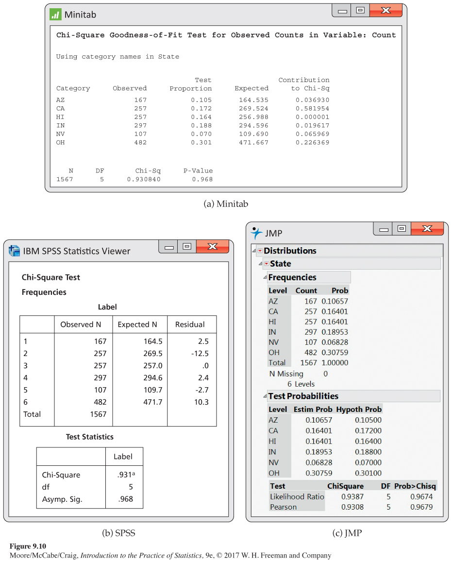
EXAMPLE 9.15
The goodness-
that the residual reported by SPSS is the numerator of this ratio. The chi-
Some software packages do not provide routines for computing the chi-
549
USE YOUR KNOWLEDGE
Question 9.32
9.32 Distribution of M&M colors. M&M Mars Company has varied the mix of colors for M&M’S Plain Chocolate Candies over the years. These changes in color blends are the result of consumer preference tests. Most recently, the color distribution is reported to be 13% brown, 14% yellow, 13% red, 20% orange, 24% blue, and 16% green.11 You open up a 14-
EXAMPLE 9.16
The sign test as a goodness-
To look at these data from the viewpoint of goodness of fit, we think of the data as two counts: patients who had a greater number of aggressive behaviors on moon days and patients who had a greater number of aggressive behaviors on other days.
550
| Counts | ||
| Moon | Other | Total |
| 14 | 1 | 15 |
If the two outcomes are equally likely, the expected counts are both 7.5 (). The expected counts are both greater than 5, so we can proceed with the significance test.
The test statistic is
We have so the degrees of freedom are 1. From Table F, we conclude that
The sign test can test the null hypothesis versus the one-