9.38 Translate each problem into a table. In each of the following scenarios, translate the problem into one that can be analyzed using a table. Give the values of and , the table, and its entries.

9.39 Sexual harassment online or in person. In the study described in Exercise 9.25, the students were also asked whether or not they were harassed in person and whether or not they were harassed online. Here are the data for the girls:

9.40 Data for the boys. Refer to the previous exercise. Here are the corresponding data for boys:

Using these data, repeat the analyses that you performed for the girls in Exercise 9.39. How do the results for the boys differ from those that you found for girls?

9.41 Repeat your analysis. In part (a) of Exercise 9.39, you had to decide which variable was explanatory and which variable was response when you computed the proportions to be compared.

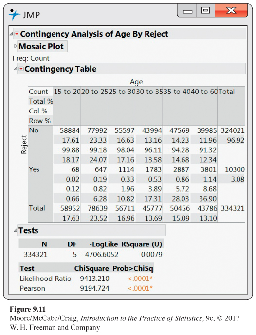
9.42 Read the output for teeth. Exercise 8.62 (page 520) gives data on individuals rejected for military service in the Cuban War of Independence in 1898 because they did not have enough teeth. In that exercise, you compared the rejection rate for those under the age of 20 with the rejection rate for those over 40. Figure 9.11 gives software output for the table that classifies the recruits into six age categories. Use the output to find the joint distribution, the marginal distributions, and the conditional distributions for these data.

9.43 Is the die fair? You suspect that a die has been altered so that the outcomes of a roll, the numbers 1 to 6, are not equally likely. You toss the die 600 times and obtain the following results:

Compute the expected counts that you would need to use in a goodness-of-fit test for these data.

9.44 Perform the significance test Refer to the previous exercise. Find the chi-square test statistic and its -value and write a short summary of your conclusions.

9.45 Health care fraud. Most errors in billing insurance providers for health care services involve honest mistakes by patients, physicians, or others involved in the health care system. However, fraud is a serious problem. The National Health Care Anti-fraud Association estimates that approximately $68 billion is lost to health care fraud each year.¹² When fraud is suspected, an audit of randomly selected billings is often conducted. The selected claims are then reviewed by experts, and each claim is classified as allowed or not allowed. The distributions of the amounts of claims are frequently highly skewed, with a large number of small claims and a small number of large claims. Because simple random sampling would likely be overwhelmed by small claims and would tend to miss the large claims, stratification is often used. See the section on stratified sampling in Chapter 3 (page 195). Here are data from an audit that used three strata based on the sizes of the claims (small, medium, and large):¹³

9.46 Population estimates. Refer to the previous exercise. One reason to do an audit such as this is to estimate the number of claims that would not be allowed if all claims in a population were examined by experts. We have an estimate of the proportion of unallowed claims from each stratum based on our sample. We know the corresponding population proportion for each stratum. Therefore, if we take the sample proportions of unallowed claims and multiply by the population sizes, we would have the estimates that we need. Here are the population sizes for the three strata:

9.47 DFW rates. One measure of student success for colleges and universities is the percent of admitted students who graduate. Studies indicate that a key issue in retaining students is their performance in so-called gateway courses. These are courses that serve as prerequisites for other key courses that are essential for student success. One measure of student performance in these courses is the DFW rate, the percent of students who receive grades of D, F, or W (withdraw). A major project was undertaken to improve the DFW rate in a gateway course at a large midwestern university. The course curriculum was revised to make it more relevant to the majors of the students taking the course, a small group of excellent teachers taught the course, technology (including clickers and online homework) was introduced, and student support outside of the classroom was increased. The following table gives data on the DFW rates for the course over three years.¹⁴ In Year 1, the traditional course was given; in Year 2, a few changes were introduced; and in Year 3, the course was substantially revised.

Do you think that the changes in this gateway course had an impact on the DFW rate? Write a report giving your answer to this question. Support your answer by an analysis of the data.

9.48 Lying to a teacher. One of the questions in a survey of high school students asked about lying to teachers.¹⁵ The following table gives the numbers of students who said that they lied to a teacher at least once during the past year, classified by sex:

9.49 When do Canadian students enter private career colleges? A survey of 13,364 Canadian students who enrolled in private career colleges was conducted to understand student participation in the private, postsecondary educational system.¹⁶ In one part of the survey, students were asked about their field of study and about when they entered college. Here are the results:

In this table, the second column gives the number of students in each field of study. The next two columns give the marginal distribution of time of entry for each field of study.

9.50 Government loans for Canadian students in private career colleges. Refer to the previous exercise. The survey also asked about how these college students paid for their education. A major source of funding was government loans. Here are the survey percents of Canadian private students who use government loans to finance their education by field of study:

9.51 Are Mexican Americans less likely to be selected as jurors? Refer to Exercise 8.97 (page 524) concerning Castaneda v. Partida, the case where the Supreme Court review used the phrase “two or three standard deviations” as a criterion for statistical significance. Recall that there were 181,535 persons eligible for jury duty, of whom 143,611 were Mexican Americans. Of the 870 people selected for jury duty, 339 were Mexican Americans. We are interested in finding out if there is an association between being a Mexican American and being selected as a juror. Formulate this problem using a two-way table of counts. Construct the table using the variables Mexican American or not and juror or not. Find the statistic and its -value. Square the statistic that you obtained in Exercise 8.97 and verify that the result is equal to the statistic.

9.52 Goodness of fit to the uniform distribution. Computer software generated 500 random numbers that should look as if they are from the uniform distribution on the interval 0 to 1 (see p. 240). They are categorized into five groups: (1) less than or equal to , (2) greater than and less than or equal to , (3) greater than and less than or equal to , (4) greater than and less than or equal to , and (5) greater than . The counts in the five groups are 114, 92, 108, 101, and 85, respectively. The probabilities for these five intervals are all the same. What is this probability? Compute the expected number for each interval for a sample of 500. Finally, perform the goodness of fit test and summarize your results.

9.53 More on goodness of fit to the uniform distribution. Refer to the previous exercise. Use software to generate your own sample of 800 uniform random variables on the interval from 0 to 1, and perform the goodness of fit test. Choose a different set of intervals than the ones used in the previous exercise.

9.54 Suspicious results? An instructor who assigned an exercise similar to the one described in the previous exercise received homework from a student who reported a -value of 0.999. The instructor suspected that the student did not use the computer for the assignment but just made up some numbers for the homework. Why was the instructor suspicious? How would this scenario change if there were 2000 students in the class?

9.55 Is there a random distribution of trees? In Example 6.1 (page 342), we examined data concerning the longleaf pine trees in the Wade Tract and concluded that the distribution of trees in the tract was not random. Here is another way to examine the same question. First, we divide the tract into four equal parts, or quadrants, in the east–west direction. Call the four parts through . Then we take a random sample of 100 trees and count the number of trees in each quadrant. Here are the data:

9.56 McNemar’s test. In Exercise 9.39 (page 551), you examined the relationship between being harassed online and being harassed in person for a sample of 1002 girls. An additional question can be asked about these data. Suppose we wanted to compare the proportions of girls who were harassed online and the proportion who were harassed in person. This is very much like the type of question that we studied in Section 8.2 (page 505). There, however, we used the assumption that the two samples used to calculate the proportions were independent. This assumption is not valid for our harassment data because the proportions are calculated from data provided by the same girls. McNemar’s test is the recommended procedure. The null hypothesis is that the two population proportions are equal and the alternative is two-sided. The test examines the counts in the cells where the two responses do not agree. In our case, these are 200 and 40. Note that if these two counts are equal, then the proportions will be equal for any possible values of counts in the other two cells. McNemar’s test is equivalent to the goodness-of-fit test that we examined in Example 9.16. Find the sample proportions, report the results of the significance test, and write a short summary of your conclusions.