Trade-
The 2000 hit movie Cast Away, starring Tom Hanks, was an update of the classic story of Robinson Crusoe, the hero of Daniel Defoe’s eighteenth-
You make a trade-
One of the important principles of economics we introduced in Module 1 was that resources are scarce. As a result, any economy—
17
The production possibilities curve illustrates the trade-
To think about the trade-
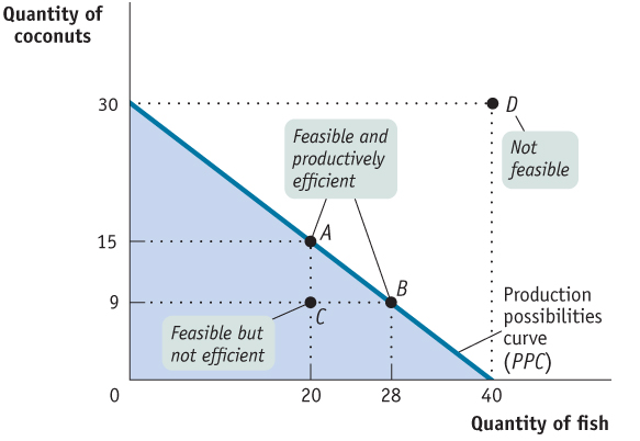
Figure 3.1 shows a hypothetical production possibilities curve for Tom, a castaway alone on an island, who must make a trade-
AP® Exam Tip
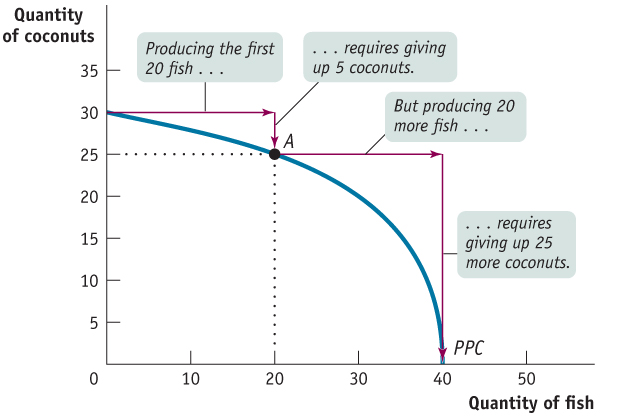
Be prepared to draw a correctly labeled production possibilities curve and use it to identify opportunity cost, efficient points, inefficient points, and unattainable points. Unemployment results in production at a point below the production possibilities curve. Most production possibilities curves are concave to the origin, as shown in Figure 3.2, due to the specialization of resources.
There is a crucial distinction between points inside or on the production possibilities curve (the shaded area) and points outside the production possibilities curve. If a production point lies inside or on the curve—
In Figure 3.1 the production possibilities curve intersects the horizontal axis at 40 fish. This means that if Tom devoted all his resources to catching fish, he would catch 40 fish per week but would have no resources left over to gather coconuts. The production possibilities curve intersects the vertical axis at 30 coconuts. This means that if Tom devoted all his resources to gathering coconuts, he could gather 30 coconuts per week but would have no resources left over to catch fish. Thus, if Tom wants 30 coconuts, the trade-
The curve also shows less extreme trade-
Thinking in terms of a production possibilities curve simplifies the complexities of reality. The real-
Efficiency
An economy is efficient if there is no way to make anyone better off without making at least one person worse off.
18
The production possibilities curve is useful for illustrating the general economic concept of efficiency. An economy is efficient if there are no missed opportunities—
An economy achieves productive efficiency if it produces at a point on its production possibilities curve.
Returning to our castaway example, as long as Tom produces a combination of coconuts and fish that is on the production possibilities curve, his production is efficient. At point A, the 15 coconuts he gathers are the maximum quantity he can get given that he has chosen to catch 20 fish; at point B, the 9 coconuts he gathers are the maximum he can get given his choice to catch 28 fish; and so on. If an economy is producing at a point on its production possibilities curve, we say that the economy has achieved productive efficiency.
But suppose that for some reason Tom was at point C, producing 20 fish and 9 coconuts. Then this one-

Another example of inefficiency in production occurs when people in an economy are involuntarily unemployed: they want to work but are unable to find jobs. When that happens, the economy is not productively efficient because it could produce more output if those people were employed. The production possibilities curve shows the amount that can possibly be produced if all resources are fully employed. In other words, changes in unemployment move the economy closer to, or further away from, the production possibilities curve (PPC). But the curve itself is determined by what would be possible if there were no unemployment in the economy. Greater unemployment is represented by points farther below the PPC—the economy is not reaching its possibilities if it is not using all of its resources. Lower unemployment is represented by points closer to the PPC—as unemployment decreases, the economy moves closer to reaching its possibilities.
An economy achieves allocative efficiency if it produces at the point along its production possibilities curve that makes consumers as well off as possible.
Although the production possibilities curve helps clarify what it means for an economy to achieve productive efficiency, it’s important to understand that productive efficiency is only part of what’s required for the economy as a whole to be efficient. Efficiency also requires that the economy allocate its resources so that consumers are as well off as possible. If an economy does this, we say that it has achieved allocative efficiency. To see why allocative efficiency is as important as productive efficiency, notice that points A and B in Figure 3.1 both represent situations in which the economy is productively efficient, because in each case it can’t produce more of one good without producing less of the other. But these two situations may not be equally desirable. Suppose that Tom prefers point B to point A—that is, he would rather consume 28 fish and 9 coconuts than 20 fish and 15 coconuts. Then point A is inefficient from the point of view of the economy as a whole: it’s possible to make Tom better off without making anyone else worse off. (Of course, in this castaway economy there isn’t anyone else; Tom is all alone.)

This example shows that efficiency for the economy as a whole requires both productive and allocative efficiency. To be efficient, an economy must produce as much of each good as it can, given the production of other goods, and it must also produce the mix of goods that people want to consume.
Opportunity Cost
19
AP® Exam Tip
Opportunity Cost = Opportunity Lost (The financial or nonfinancial cost of a choice not taken.)
The production possibilities curve is also useful as a reminder that the true cost of any good is not only its price, but also everything else in addition to money that must be given up in order to get that good—
Is the opportunity cost of an extra fish in terms of coconuts always the same, no matter how many fish Tom catches? In the example illustrated by Figure 3.1, the answer is yes. If Tom increases his catch from 28 to 40 fish, an increase of 12, the number of coconuts he gathers falls from 9 to zero. So his opportunity cost per additional fish is 9⁄12 = 3⁄4 of a coconut, the same as it was when his catch went from 20 fish to 28. However, the fact that in this example the opportunity cost of an additional fish in terms of coconuts is always the same is a result of an assumption we’ve made, an assumption that’s reflected in the way Figure 3.1 is drawn. Specifically, whenever we assume that the opportunity cost of an additional unit of a good doesn’t change regardless of the output mix, the production possibilities curve is a straight line.
Moreover, as you might have already guessed, the slope of a straight-
Figure 3.2 illustrates a different assumption, a case in which Tom faces increasing opportunity cost. Here, the more fish he catches, the more coconuts he has to give up to catch an additional fish, and vice versa. For example, to go from producing zero fish to producing 20 fish, he has to give up 5 coconuts. That is, the opportunity cost of those 20 fish is 5 coconuts. But to increase his fish production from 20 to 40—
20
Although it’s often useful to work with the simple assumption that the production possibilities curve is a straight line, economists believe that in reality, opportunity costs are typically increasing. When only a small amount of a good is produced, the opportunity cost of producing that good is relatively low because the economy needs to use only those resources that are especially well suited for its production. For example, if an economy grows only a small amount of corn, that corn can be grown in places where the soil and climate are perfect for growing corn but less suitable for growing anything else, such as wheat. So growing that corn involves giving up only a small amount of potential wheat output. Once the economy grows a lot of corn, however, land that is well suited for wheat but isn’t so great for corn must be used to produce corn anyway. As a result, the additional corn production involves sacrificing considerably more wheat production. In other words, as more of a good is produced, its opportunity cost typically rises because well-
Economic Growth
Finally, the production possibilities curve helps us understand what it means to talk about economic growth. We introduced the concept of economic growth in Module 2, saying that it allows a sustained rise in aggregate output. We learned that economic growth is one of the fundamental features of the economy. But are we really justified in saying that the economy has grown over time? After all, although the U.S. economy produces more of many things than it did a century ago, it produces less of other things—
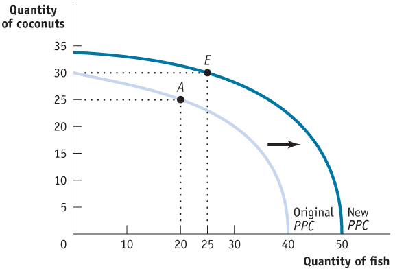
The answer, illustrated in Figure 3.3, is that economic growth means an expansion of the economy’s production possibilities: the economy can produce more of everything. For example, if Tom’s production is initially at point A (20 fish and 25 coconuts), economic growth means that he could move to point E (25 fish and 30 coconuts). Point E lies outside the original curve, so in the production possibilities curve model, growth is shown as an outward shift of the curve. Unless the PPC shifts outward, the points beyond the PPC are unattainable. Those points beyond a given PPC are beyond the economy’s possibilities.
21
What can cause the production possibilities curve to shift outward? There are two general sources of economic growth. One is an increase in the resources used to produce goods and services: labor, land, capital, and entrepreneurship. To see how adding to an economy’s resources leads to economic growth, suppose that Tom finds a fishing net washed ashore on the beach. The fishing net is a resource he can use to produce more fish in the course of a day spent fishing. We can’t say how many more fish Tom will catch; that depends on how much time he decides to spend fishing now that he has the net. But because the net makes his fishing more productive, he can catch more fish without reducing the number of coconuts he gathers, or he can gather more coconuts without reducing his fish catch. So his production possibilities curve shifts outward.
Technology is the technical means for producing goods and services.
The other source of economic growth is progress in technology, the technical means for the production of goods and services. Suppose Tom figures out a better way either to catch fish or to gather coconuts—
Again, economic growth means an increase in what the economy can produce. What the economy actually produces depends on the choices people make. After his production possibilities expand, Tom might not choose to produce both more fish and more coconuts; he might choose to increase production of only one good, or he might even choose to produce less of one good. For example, if he gets better at catching fish, he might decide to go on an all-
The production possibilities curve is a very simplified model of an economy, yet it teaches us important lessons about real-