The Role of the Exchange Rate
We’ve just seen how differences in the supply of loanable funds from savings and the demand for loanable funds for investment spending lead to international capital flows. We’ve also learned that a country’s balance of payments on the current account plus its balance of payments on the financial account add up to zero: a country that receives net capital inflows must run a matching current account deficit, and a country that generates net capital outflows must run a matching current account surplus.
AP® Exam Tip
The foreign exchange market appears frequently on the AP® exam. You may be expected to graph and explain this market in the free-
The behavior of the financial account—
The answer lies in the role of the exchange rate, which is determined in the foreign exchange market.
Understanding Exchange Rates
In general, goods, services, and assets produced in a country must be paid for in that country’s currency. U.S. products must be paid for in dollars; most European products must be paid for in euros; Japanese products must be paid for in yen. Occasionally, sellers will accept payment in foreign currency, but they will then exchange that currency for domestic money.
Currencies are traded in the foreign exchange market.
The prices at which currencies trade are known as exchange rates.
International transactions, then, require a market—
418
Table 42.1 shows exchange rates among the world’s three most important currencies as of 12:50 A.M., EST, on April 3, 2014. Each entry shows the price of the “row” currency in terms of the “column” currency. For example, at that time US$1 exchanged for €0.7269, so it took €0.7269 to buy US$1. Similarly, it took US$1.3757 to buy €1. These two numbers reflect the same rate of exchange between the euro and the U.S. dollar: 1/1.3757 = €0.7269.
Table 42.1Exchange Rates, April 3, 2014, 12:50 A.M.
| U.S. dollars | Yen | Euros | |
| One U.S. dollar exchanged for | 1 | 103.97 | 0.7269 |
| One yen exchanged for | 0.0096 | 1 | 0.007 |
| One euro exchanged for | 1.3757 | 143.04 | 1 |
There are two ways to write any given exchange rate. In this case, there were €0.7269 to US$1 and US$1.3757 to €1. Which is the correct way to write it? The answer is that there is no fixed rule. In most countries, people tend to express the exchange rate as the price of a dollar in domestic currency. However, this rule isn’t universal, and the U.S. dollar–
When a currency becomes more valuable in terms of other currencies, it appreciates.
When a currency becomes less valuable in terms of other currencies, it depreciates.
When discussing movements in exchange rates, economists use specialized terms to avoid confusion. When a currency becomes more valuable in terms of other currencies, economists say that the currency appreciates. When a currency becomes less valuable in terms of other currencies, it depreciates. Suppose, for example, that the value of €1 went from $1 to $1.25, which means that the value of US$1 went from €1 to €0.80 (because 1/1.25 = 0.80). In this case, we would say that the euro appreciated and the U.S. dollar depreciated.
Movements in exchange rates, other things equal, affect the relative prices of goods, services, and assets in different countries. Suppose, for example, that the price of an American hotel room is US$100 and the price of a French hotel room is €100. If the exchange rate is €1 = US$1, these hotel rooms have the same price. If the exchange rate is €1.25 = US$1, however, the French hotel room is 20% cheaper than the American hotel room. If the exchange rate is €0.80 = US$1, the French hotel room is 25% more expensive than the American hotel room.
But what determines exchange rates? Supply and demand in the foreign exchange market.
The Equilibrium Exchange Rate
For the sake of simplicity, imagine that there are only two currencies in the world: U.S. dollars and euros. Europeans who want to purchase American goods, services, and assets come to the foreign exchange market to exchange euros for U.S. dollars. That is, Europeans demand U.S. dollars from the foreign exchange market and, correspondingly, supply euros to that market. Americans who want to buy European goods, services, and assets come to the foreign exchange market to exchange U.S. dollars for euros. That is, Americans supply U.S. dollars to the foreign exchange market and, correspondingly, demand euros from that market. International transfers and payments of factor income also enter into the foreign exchange market, but to make things simple, we’ll ignore these.
Figure 42.1 shows how the foreign exchange market works. The quantity of dollars demanded and supplied at any given euro–
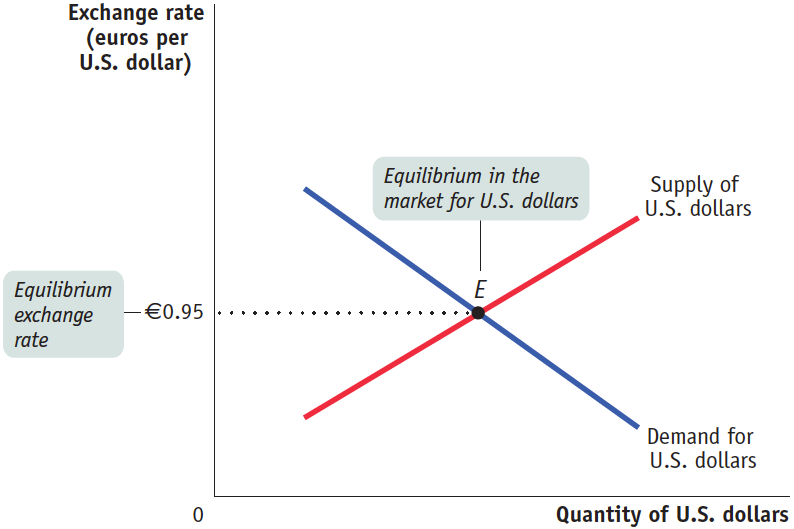
The figure shows two curves, the demand curve for U.S. dollars and the supply curve for U.S. dollars. The key to understanding the slopes of these curves is that the level of the exchange rate affects exports and imports. When a country’s currency appreciates (becomes more valuable), exports fall and imports rise. When a country’s currency depreciates (becomes less valuable), exports rise and imports fall. To understand why the demand curve for U.S. dollars slopes downward, recall that the exchange rate, other things equal, determines the prices of American goods, services, and assets relative to those of European goods, services, and assets. If the U.S. dollar rises against the euro (the dollar appreciates), American products will become more expensive to Europeans relative to European products. So Europeans will buy less from the United States and will acquire fewer dollars in the foreign exchange market: the quantity of U.S. dollars demanded falls as the number of euros needed to buy a U.S. dollar rises. If the U.S. dollar falls against the euro (the dollar depreciates), American products will become relatively cheaper for Europeans. Europeans will respond by buying more from the United States and acquiring more dollars in the foreign exchange market: the quantity of U.S. dollars demanded rises as the number of euros needed to buy a U.S. dollar falls.
419
A similar argument explains why the supply curve of U.S. dollars in Figure 42.1 slopes upward: the more euros required to buy a U.S. dollar, the more dollars Americans will supply. Again, the reason is the effect of the exchange rate on relative prices. If the U.S. dollar rises against the euro, European products look cheaper to Americans—
The equilibrium exchange rate is the exchange rate at which the quantity of a currency demanded in the foreign exchange market is equal to the quantity supplied.
The equilibrium exchange rate is the exchange rate at which the quantity of U.S. dollars demanded in the foreign exchange market is equal to the quantity of U.S. dollars supplied. In Figure 42.1, the equilibrium is at point E, and the equilibrium exchange rate is 0.95. That is, at an exchange rate of €0.95 per US$1, the quantity of U.S. dollars supplied to the foreign exchange market is equal to the quantity of U.S. dollars demanded.
To understand the significance of the equilibrium exchange rate, it’s helpful to consider a numerical example of what equilibrium in the foreign exchange market looks like. Such an example is shown in Table 42.2. (This is a hypothetical table that isn’t intended to match real numbers.) The first row shows European purchases of U.S. dollars, either to buy U.S. goods and services or to buy U.S. assets such as real estate or shares of stock in U.S. companies. The second row shows U.S. sales of U.S. dollars, either to buy European goods and services or to buy European assets. At the equilibrium exchange rate, the total quantity of U.S. dollars Europeans want to buy is equal to the total quantity of U.S. dollars Americans want to sell.
Table 42.2Equilibrium in the Foreign Exchange Market: A Hypothetical Example
| European purchases of U.S. dollars (trillions of U.S. dollars) | To buy U.S. goods and services: 1.0 | To buy U.S. assets: 1.0 | Total purchases of U.S. dollars: 2.0 |
| U.S. sales of U.S. dollars (trillions of U.S. dollars) | To buy European goods and services: 1.5 | To buy European assets: 0.5 | Total sales of U.S. dollars: 2.0 |
| U.S. balance of payments on the current account: −0.5 | U.S. balance of payments on the financial account: +0.5 |
Remember that the balance of payments accounts divide international transactions into two types. Purchases and sales of goods and services are counted in the current account. (Again, we’re leaving out transfers and factor income to keep things simple.) Purchases and sales of assets are counted in the financial account. At the equilibrium exchange rate, then, we have the situation shown in Table 42.2: the sum of the balance of payments on the current account plus the balance of payments on the financial account is zero.
420
Now let’s briefly consider how a shift in the demand for U.S. dollars affects equilibrium in the foreign exchange market. Suppose that for some reason capital flows from Europe to the United States increase—
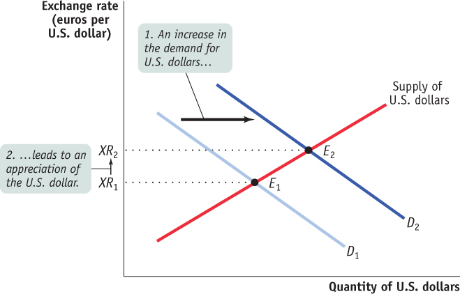
What are the consequences of this increased capital inflow for the balance of payments? The total quantity of U.S. dollars supplied to the foreign exchange market still must equal the total quantity of U.S. dollars demanded. So the increased capital inflow to the United States—
Table 42.3 shows how this might work. Europeans are buying more U.S. assets, increasing the balance of payments on the financial account from 0.5 to 1.0. This is offset by a reduction in European purchases of U.S. goods and services and a rise in U.S. purchases of European goods and services, both the result of the dollar’s appreciation. So any change in the U.S. balance of payments on the financial account generates an equal and opposite reaction in the balance of payments on the current account. Movements in the exchange rate ensure that changes in the financial account and in the current account offset each other.
421
Table 42.3Effects of Increased Capital Inflows
| European purchases of U.S. dollars (trillions of U.S. dollars) | To buy U.S. goods and services: 0.75 (down 0.25) | To buy U.S. assets: 1.5 (up 0.5) | Total purchases of U.S. dollars: 2.25 |
| U.S. sales of U.S. dollars (trillions of U.S. dollars) | To buy European goods and services: 1.75 (up 0.25) | To buy European assets: 0.5 (no change) | Total sales of U.S. dollars: 2.25 |
| U.S. balance of payments on the current account: −1.0 (down 0.5) | U.S. balance of payments on the financial account: +1.0 (up 0.5) |
Let’s briefly run this process in reverse. Suppose there is a reduction in capital flows from Europe to the United States—
Inflation and Real Exchange Rates
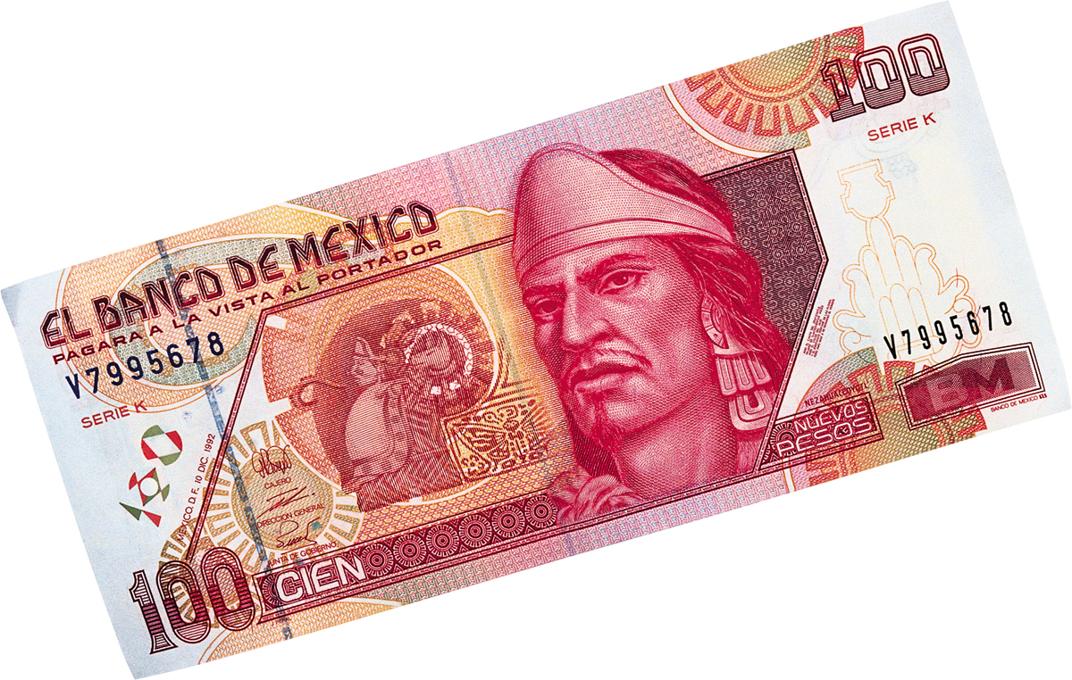
In 1994, on average, one U.S. dollar exchanged for 3.4 Mexican pesos. By 2014, the peso had fallen against the dollar by almost 75%, with an average exchange rate in early 2014 of 13.3 pesos per dollar. Did Mexican products also become much cheaper relative to U.S. products over that 20-
Real exchange rates are exchange rates adjusted for international differences in aggregate price levels.
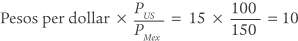
To take account of the effects of differences in inflation rates, economists calculate real exchange rates, exchange rates adjusted for international differences in aggregate price levels. Suppose that the exchange rate we are looking at is the number of Mexican pesos per U.S. dollar. Let PUS and PMex be indexes of the aggregate price levels in the United States and Mexico, respectively. Then the real exchange rate between the Mexican peso and the U.S. dollar is defined as:

To distinguish it from the real exchange rate, the exchange rate unadjusted for aggregate price levels is sometimes called the nominal exchange rate.
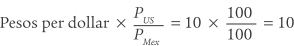
To understand the significance of the difference between the real and nominal exchange rates, let’s consider the following example. Suppose that the Mexican peso depreciates against the U.S. dollar, with the exchange rate going from 10 pesos per U.S. dollar to 15 pesos per U.S. dollar, a 50% change. But suppose that at the same time the price of everything in Mexico, measured in pesos, increases by 50%, so that the Mexican price index rises from 100 to 150. We’ll assume that there is no change in U.S. prices, so that the U.S. price index remains at 100. The initial real exchange rate is:
422
After the peso depreciates and the Mexican price level increases, the real exchange rate is:
In this example, the peso has depreciated substantially in terms of the U.S. dollar, but the real exchange rate between the peso and the U.S. dollar hasn’t changed at all. And because the real peso–
The same is true for all goods and services that enter into trade: the current account responds only to changes in the real exchange rate, not the nominal exchange rate. A country’s products become cheaper to foreigners only when that country’s currency depreciates in real terms, and those products become more expensive to foreigners only when the currency appreciates in real terms. As a consequence, economists who analyze movements in exports and imports of goods and services focus on the real exchange rate, not the nominal exchange rate.
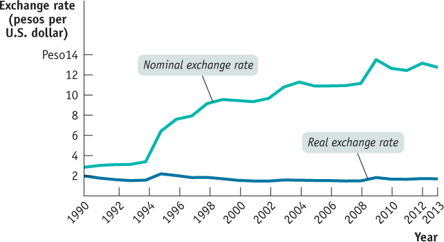
Figure 42.3 illustrates just how important it can be to distinguish between nominal and real exchange rates. The line labeled “Nominal exchange rate” shows the number of pesos exchanged for a U.S. dollar from 1990 to 2013. As you can see, the peso depreciated massively over that period. But the line labeled “Real exchange rate” indicates the cost of Mexican products to U.S. consumers: it was calculated using Equation 42.1, with price indexes for both Mexico and the United States set so that the value in 1990 was 100. In real terms, the peso depreciated between 1994 and 1995, and again in 2008, but not by nearly as much as the nominal depreciation. By 2013, the real peso–
Purchasing Power Parity
423
The purchasing power parity between two countries’ currencies is the nominal exchange rate at which a given basket of goods and services would cost the same amount in each country.
A useful tool for analyzing exchange rates, closely connected to the concept of the real exchange rate, is known as purchasing power parity. The purchasing power parity between two countries’ currencies is the nominal exchange rate at which a given basket of goods and services would cost the same amount in each country. For example, suppose that a basket of goods and services that costs $100 in the United States costs 1,000 pesos in Mexico. Then the purchasing power parity is 10 pesos per U.S. dollar: at that exchange rate, 1,000 pesos = $100, so the market basket costs the same amount in both countries.
Calculations of purchasing power parities are usually made by estimating the cost of buying broad market baskets containing many goods and services—
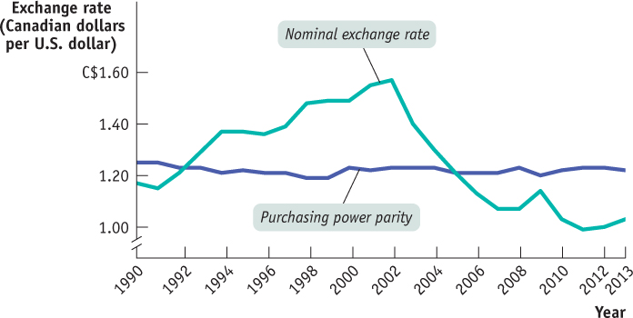
Nominal exchange rates almost always differ from purchasing power parities. Some of these differences are systematic: in general, aggregate price levels are lower in poor countries than in rich countries because services tend to be cheaper in poor countries. But even among countries at roughly the same level of economic development, nominal exchange rates vary quite a lot from purchasing power parity. Figure 42.4 shows the nominal exchange rate between the Canadian dollar and the U.S. dollar, measured as the number of Canadian dollars per U.S. dollar, from 1990 to 2013, together with an estimate of the purchasing power parity exchange rate between the United States and Canada over the same period. The purchasing power parity didn’t change much over the whole period because the United States and Canada had about the same rate of inflation. But at the beginning of the period the nominal exchange rate was below purchasing power parity, so a given market basket was more expensive in Canada than in the United States. By 2002, the nominal exchange rate was far above the purchasing power parity, so a market basket was much cheaper in Canada than in the United States.
Over the long run, however, purchasing power parities are pretty good at predicting actual changes in nominal exchange rates. In particular, nominal exchange rates between countries at similar levels of economic development tend to fluctuate around levels that lead to similar costs for a given market basket. In fact, by July 2005, the nominal exchange rate between the United States and Canada was C$1.22 per US$1—
Burgernomics
For a number of years the British magazine The Economist has produced an annual comparison of the cost in different countries of one particular consumption item that is found around the world—

In the January 2014 version of the Big Mac index, there were some wide variations in the dollar price of a Big Mac. In the U.S., the price was $4.62. In China, converting at the official exchange rate, a Big Mac cost only $2.74. In Switzerland, though, the price was $7.14.
The Big Mac index suggested that the euro would eventually fall against the dollar: a Big Mac on average cost €3.66, so that the purchasing power parity was $1.26 per €1 versus an actual market exchange rate of $1.38.
Serious economic studies of purchasing power parity require data on the prices of many goods and services. However, it turns out that estimates of purchasing power parity based on the Big Mac index usually aren’t that different from more elaborate measures. Fast food seems to make for pretty good fast research.
424
Low-Cost America
Interest Rates and the U.S. Housing Boom
Does the exchange rate matter for business decisions? And how. Consider what European auto manufacturers were doing in 2008. One report from the University of Iowa summarized the situation as follows:
“While luxury German carmakers BMW and Mercedes have maintained plants in the American South since the 1990s, BMW aims to expand U.S. manufacturing in South Carolina by 50% during the next five years. Volvo of Sweden is in negotiations to build a plant in New Mexico. Analysts at Italian carmaker Fiat determined that it needs to build a North American factory to profit from the upcoming re-
Why were European automakers flocking to America? To some extent because they were being offered special incentives, as the case of Volkswagen in Tennessee illustrates. But the big factor was the exchange rate. In the early 2000s, on average, one euro was worth less than a dollar; by the summer of 2008 the exchange rate was around €1 = $1.50. This change in the exchange rate made it substantially cheaper for European car manufacturers to produce in the United States than at home—
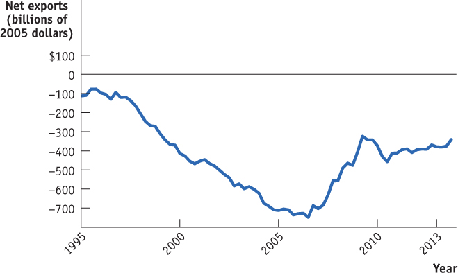
Automobile manufacturing wasn’t the only U.S. industry benefiting from the weak dollar; across the board, U.S. exports surged after 2006 while import growth fell off. The figure shows one measure of U.S. trade performance, real net exports of goods and services: exports minus imports, both measured in 2005 dollars. As you can see, this balance, after a long slide, turned sharply upward in 2006.
There was a modest reversal in 2009–