What the Price Elasticity of Demand Tells Us
Med-
How Elastic Is Elastic?
Demand is perfectly inelastic when the quantity demanded does not respond at all to changes in the price. When demand is perfectly inelastic, the demand curve is a vertical line.
As a first step toward classifying price elasticities of demand, let’s look at the extreme cases.
First, consider the demand for a good when people pay no attention to its price. Suppose, for example, that consumers would buy 1 billion pairs of shoelaces per year regardless of the price. If that were true, the demand curve for shoelaces would look like the curve shown in panel (a) of Figure 47.1: it would be a vertical line at 1 billion pairs of shoelaces. Since the percent change in the quantity demanded is zero for any change in the price, the price elasticity of demand in this case is zero. The case of a zero price elasticity of demand is known as perfectly inelastic demand.
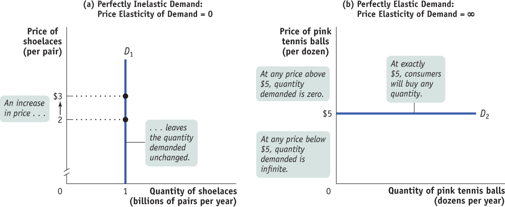
Demand is perfectly elastic when any price increase will cause the quantity demanded to drop to zero. When demand is perfectly elastic, the demand curve is a horizontal line.
Demand is elastic if the price elasticity of demand is greater than 1, inelastic if the price elasticity of demand is less than 1, and unit-
The opposite extreme occurs when even a tiny rise in the price will cause the quantity demanded to drop to zero or even a tiny fall in the price will cause the quantity demanded to get extremely large. Panel (b) of Figure 47.1 shows the case of pink tennis balls; we suppose that tennis players really don’t care what color their balls are and that other colors, such as neon green and vivid yellow, are available at $5 per dozen balls. In this case, consumers will buy no pink balls if they cost more than $5 per dozen but will buy only pink balls if they cost less than $5. The demand curve will therefore be a horizontal line at a price of $5 per dozen balls. As you move back and forth along this line, there is a change in the quantity demanded but no change in the price. When you divide a number by zero, you get infinity, denoted by the symbol ∞. So a horizontal demand curve implies an infinite price elasticity of demand. When the price elasticity of demand is infinite, economists say that demand is perfectly elastic.
468
The price elasticity of demand for the vast majority of goods is somewhere between these two extreme cases. Economists use one main criterion for classifying these intermediate cases: they ask whether the price elasticity of demand is greater or less than 1. When the price elasticity of demand is greater than 1, economists say that demand is elastic. When the price elasticity of demand is less than 1, they say that demand is inelastic. The borderline case is unit-
To see why a price elasticity of demand equal to 1 is a useful dividing line, let’s consider a hypothetical example: a toll bridge operated by the state highway department. Other things equal, the number of drivers who use the bridge depends on the toll, the price the highway department charges for crossing the bridge: the higher the toll, the fewer the drivers who use the bridge.
469
Figure 47.2 shows three hypothetical demand curves that exhibit unit-
AP® Exam Tip
When thinking of perfectly inelastic demand, think I = Inelastic, with the I representing the vertical perfectly inelastic demand curve. When thinking of perfectly elastic demand, think E = Elastic, with the horizontal middle line of the E representing the horizontal perfectly elastic demand curve.
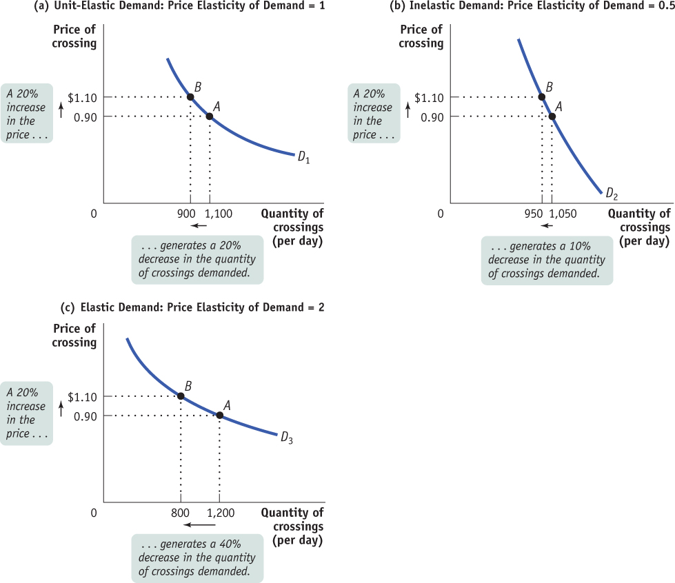
Panel (a) shows what happens when the toll is raised from $0.90 to $1.10 and the demand curve is unit-
Panel (b) shows a case of inelastic demand when the toll is raised from $0.90 to $1.10. The same 20% increase in price reduces the quantity demanded from 1,050 to 950. That’s only a 10% decline, so in this case the price elasticity of demand is 10%/20% = 0.5.
Panel (c) shows a case of elastic demand when the toll is raised from $0.90 to $1.10. The 20% price increase causes the quantity demanded to fall from 1,200 to 800, a 40% decline, so the price elasticity of demand is 40%/20% = 2.
470
Total revenue is the total value of sales of a good or service. It is equal to the price multiplied by the quantity sold.
Why does it matter whether demand is unit-
(47-
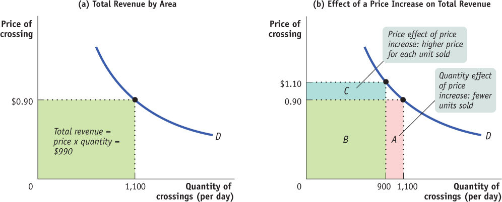
Total revenue has a useful graphical representation that can help us understand why knowing the price elasticity of demand is crucial when we ask whether an increase in price will increase or reduce total revenue. Panel (a) of Figure 47.3 shows the same demand curve as panel (a) of Figure 47.2. We see that 1,100 drivers will use the bridge if the toll is $0.90. So the total revenue at a price of $0.90 is $0.90 × 1,100 = $990. This value is equal to the area of the green rectangle, which is drawn with the bottom left corner at the point (0, 0) and the top right corner at (1,100, 0.90). In general, the total revenue at any given price is equal to the area of a rectangle whose height is the price and whose width is the quantity demanded at that price.
AP® Exam Tip
Don’t confuse revenue with profit. Revenue is what the firm receives; profit is what the firm receives minus the firm’s costs.
To get an idea of why total revenue is important, consider the following scenario. Suppose that the toll on the bridge is currently $0.90 but that the highway department must raise extra money for road repairs. One way to do this is to raise the toll on the bridge. But this plan might backfire, since a higher toll will reduce the number of drivers who use the bridge. And if traffic on the bridge dropped a lot, a higher toll would actually reduce total revenue instead of increasing it. So it’s important for the highway department to know how drivers will respond to a toll increase.
We can see graphically how the toll increase affects total bridge revenue by examining panel (b) of Figure 47.3. At a toll of $0.90, total revenue is given by the sum of areas A and B. After the toll is raised to $1.10, total revenue is given by the sum of areas B and C. So when the toll is raised, revenue represented by area A is lost but revenue represented by area C is gained. These two areas have important interpretations. Area C represents the revenue gain that comes from the additional $0.20 paid by drivers who continue to use the bridge. That is, the 900 who continue to use the bridge contribute an additional $0.20 × 900 = $180 per day to total revenue, represented by area C. But 200 drivers who would have used the bridge at a price of $0.90 no longer do so, generating a loss to total revenue of $0.90 × 200 = $180 per day, represented by area A. (In this particular example, because demand is unit-
471
Except in the rare case of a good with perfectly elastic or perfectly inelastic demand, when a seller raises the price of a good, two countervailing effects are present:
A price effect. After a price increase, each unit sold sells at a higher price, which tends to raise revenue.
A quantity effect. After a price increase, fewer units are sold, which tends to lower revenue.
But what is the net ultimate effect on total revenue: does it go up or down? The answer is that, in general, total revenue can go either way—
The price elasticity of demand tells us what happens to total revenue when price changes: its size determines which effect—
AP® Exam Tip
If total revenue and price move in the same direction, the good is inelastic. If total revenue and price move in opposite directions, the good is elastic. If total revenue does not change when price changes, the good is unit-
If demand for a good is unit-
elastic (the price elasticity of demand is 1), an increase in price does not change total revenue. In this case, the quantity effect and the price effect exactly offset each other. If demand for a good is inelastic (the price elasticity of demand is less than 1), a higher price increases total revenue. In this case, the price effect is stronger than the quantity effect.
If demand for a good is elastic (the price elasticity of demand is greater than 1), an increase in price reduces total revenue. In this case, the quantity effect is stronger than the price effect.
Table 47.1 shows how the effect of a price increase on total revenue depends on the price elasticity of demand, using the same data as in Figure 47.2. An increase in the price from $0.90 to $1.10 leaves total revenue unchanged at $990 when demand is unit-
Table 47.1Price Elasticity of Demand and Total Revenue
| Price of crossing = $0.90 | Price of crossing = $1.10 | |
| Unit- |
||
| Quantity demanded | 1,100 | 0 900 |
| Total revenue | $990 | $990 |
| Inelastic demand (price elasticity of demand = 0.5) | ||
| Quantity demanded | 1,050 | $ 950 |
| Total revenue | $945 | $1,045 |
| Elastic demand (price elasticity of demand = 2) | ||
| Quantity demanded | 1,200 | 800 |
| Total revenue | $1,080 | $880 |
472
The price elasticity of demand also predicts the effect of a fall in price on total revenue. When the price falls, the same two countervailing effects are present, but they work in the opposite directions as compared to the case of an increase in price. There is the price effect of a lower price per unit sold, which tends to lower revenue. This is countered by the quantity effect of more units sold, which tends to raise revenue. Which effect dominates depends on the price elasticity. Here is a quick summary:
When demand is unit-
elastic, the two effects exactly balance each other out; so a fall in price has no effect on total revenue. When demand is inelastic, the price effect dominates the quantity effect; so a fall in price reduces total revenue.
When demand is elastic, the quantity effect dominates the price effect; so a fall in price increases total revenue.
Price Elasticity Along the Demand Curve
Suppose an economist says that “the price elasticity of demand for coffee is 0.25.” What he or she means is that at the current price the elasticity is 0.25. In the previous discussion of the toll bridge, what we were really describing was the elasticity at the price of $0.90. Why this qualification? Because for the vast majority of demand curves, the price elasticity of demand at one point along the curve is different from the price elasticity of demand at other points along the same curve.
To see this, consider the table in Figure 47.4, which shows a hypothetical demand schedule. It also shows in the last column the total revenue generated at each price. The upper panel of the graph in Figure 47.4 shows the corresponding demand curve. The lower panel illustrates the same data on total revenue: the height of a bar at each quantity demanded—
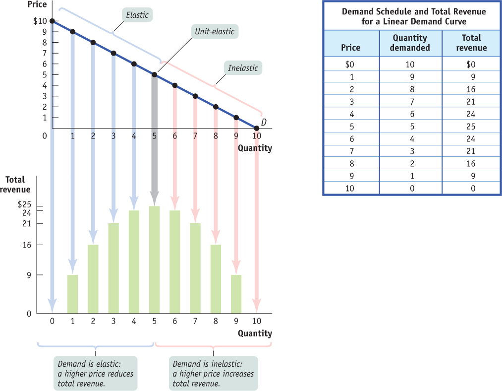
In Figure 47.4, you can see that when the price is low, raising the price increases total revenue: starting at a price of $1, raising the price to $2 increases total revenue from $9 to $16. This means that when the price is low, demand is inelastic. Moreover, you can see that demand is inelastic on the entire section of the demand curve from a price of $0 to a price of $5.
AP® Exam Tip
For a straight, downward-
When the price is high, however, raising it further reduces total revenue: starting at a price of $8, for example, raising the price to $9 reduces total revenue, from $16 to $9. This means that when the price is high, demand is elastic. Furthermore, you can see that demand is elastic over the section of the demand curve from a price of $5 to $10.
For the vast majority of goods, the price elasticity of demand changes along the demand curve. So whenever you measure a good’s elasticity, you are really measuring it at a particular point or section of the good’s demand curve.
What Factors Determine the Price Elasticity of Demand?
The flu vaccine shortfall of 2004–
473
Whether Close Substitutes Are Available The price elasticity of demand tends to be high if there are other goods that consumers regard as similar and would be willing to consume instead. The price elasticity of demand tends to be low if there are no close substitutes.

Whether the Good Is a Necessity or a Luxury The price elasticity of demand tends to be low if a good is something you must have, like a life-
Share of Income Spent on the Good The price elasticity of demand tends to be low when spending on a good accounts for a small share of a consumer’s income. In that case, a significant change in the price of the good has little impact on how much the consumer spends. In contrast, when a good accounts for a significant share of a consumer’s spending, the consumer is likely to be very responsive to a change in price. In this case, the price elasticity of demand is high.
474
Time In general, the price elasticity of demand tends to increase as consumers have more time to adjust to a price change. This means that the long-
AP® Exam Tip
The determinants of price elasticity of demand are:
S - Substitutes
P - Proportion of income
L - Luxury or necessity
A - Addictive or habit forming
T - Time
A good illustration of the effect of time on the elasticity of demand is drawn from the 1970s, the first time gasoline prices increased dramatically in the United States. Initially, consumption fell very little because there were no close substitutes for gasoline and because driving their cars was necessary for people to carry out the ordinary tasks of life. Over time, however, Americans changed their habits in ways that enabled them to gradually reduce their gasoline consumption. The result was a steady decline in gasoline consumption over the next decade, even though the price of gasoline did not continue to rise, confirming that the long-
Responding to Your Tuition Bill
College costs more than ever—
A 1988 study found that a 3% increase in tuition led to an approximately 2% fall in the number of students enrolled at four-
A 1999 study confirmed this pattern. In comparison to four-
Interestingly, the 1999 study found that for both two-
Sources: Leslie, L. L., & Brinkman, P. T. (1988). The Economic Value of Higher Education. Washington, DC: American Council on Education: Heller, D. E. (1999). The Effects of Tuition and State Financial Aid on Public College Enrollment. The Review of Higher Education, 23(1), 65–