The principle of diminishing marginal utility explains why most people eventually reach a limit, even at an all-you-can-eat buffet where the cost of another clam is measured only in future indigestion. Under ordinary circumstances, however, it costs some additional resources to consume more of a good, and consumers must take that cost into account when making choices.

What do we mean by cost? As always, the fundamental measure of cost is opportunity cost. Because the amount of money a consumer can spend is limited, a decision to consume more of one good is also a decision to consume less of some other good.

Consider Sammy, whose appetite is exclusively for clams and potatoes. (There’s no accounting for tastes.) He has a weekly income of $20 and since, given his appetite, more of either good is better than less, he spends all of it on clams and potatoes. We will assume that clams cost $4 per pound and potatoes cost $2 per pound. What are his possible choices?

Whatever Sammy chooses, we know that the cost of his consumption bundle cannot exceed the amount of money he has to spend. That is,

(51-1) Expenditure on clams + Expenditure on potatoes ≤ Total income

Consumers always have limited income, which constrains how much they can consume. So the requirement illustrated by Equation 51-1—that a consumer must choose a consumption bundle that costs no more than his or her income—is known as the consumer’s budget constraint. It’s a simple way of saying that a consumer can’t spend more than the total amount of income available to him or her. In other words, consumption bundles are affordable when they obey the budget constraint. We call the set of all of Sammy’s affordable consumption bundles his consumption possibilities. In general, whether or not a particular consumption bundle is included in a consumer’s consumption possibilities depends on the consumer’s income and the prices of goods and services.

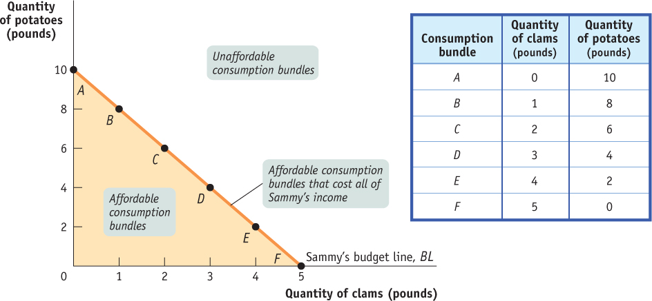
Figure 51.2 shows Sammy’s consumption possibilities. The quantity of clams in his consumption bundle is measured on the horizontal axis and the quantity of potatoes on the vertical axis. The downward-sloping line connecting points A through F shows which consumption bundles are affordable and which are not. Every bundle on or inside this line (the shaded area) is affordable; every bundle outside this line is unaffordable. As an example of one of the points, let’s look at point C, representing 2 pounds of clams and 6 pounds of potatoes, and check whether it satisfies Sammy’s budget constraint. The cost of bundle C is 6 pounds of potatoes × $2 per pound + 2 pounds of clams × $4 per pound = $12 + $8 = $20. So bundle C does indeed satisfy Sammy’s budget constraint: it costs no more than his weekly income of $20. In fact, bundle C costs exactly as much as Sammy’s income. By doing the arithmetic, you can check that all the other points lying on the downward-sloping line are also bundles at which Sammy spends all of his income.

518

The downward-sloping line has a special name, the budget line. It shows all the consumption bundles available to Sammy when he spends all of his income. It’s downward-sloping because when Sammy is spending all of his income, say by consuming at point A on the budget line, then in order to consume more clams he must consume fewer potatoes—that is, he must move to a point like B. In other words, when Sammy is on his budget line, the opportunity cost of consuming more clams is consuming fewer potatoes, and vice versa. As Figure 51.2 indicates, any consumption bundle that lies above the budget line is unaffordable.

Do we need to consider the other bundles in Sammy’s consumption possibilities—the ones that lie within the shaded region in Figure 51.2 bounded by the budget line? The answer, for all practical situations, is no: as long as Sammy doesn’t get satiated—that is, as long as his marginal utility from consuming either good is always positive—and he doesn’t get any utility from saving income rather than spending it, then he will always choose to consume a bundle that lies on his budget line.

Given that $20 per week budget, next we can consider the culinary dilemma of what point on his budget line Sammy will choose.

519

Because Sammy’s budget constrains him to a consumption bundle somewhere along the budget line, a choice to consume a given quantity of clams also determines his potato consumption, and vice versa. We want to find the consumption bundle—represented by a point on the budget line—that maximizes Sammy’s total utility. This bundle is Sammy’s optimal consumption bundle.

Table 51.1 shows hypothetical levels of utility Sammy gets from consuming various quantities of clams and potatoes, respectively. According to the table, Sammy has a healthy appetite; the more of either good he consumes, the higher his utility. But because he has a limited budget, he must make a trade-off: the more pounds of clams he consumes, the fewer pounds of potatoes, and vice versa. That is, he must choose a point on his budget line.

Table 51.2 shows how his total utility varies for the different consumption bundles along his budget line. Each of six possible consumption bundles, A through F from Figure 51.2, is given in the first column. The second column shows the level of clam consumption corresponding to each choice. The third column shows the utility Sammy gets from consuming those clams. The fourth column shows the quantity of potatoes Sammy can afford given the level of clam consumption; this quantity goes down as his clam consumption goes up because he is sliding down the budget line. The fifth column shows the utility he gets from consuming those potatoes. And the final column shows his total utility. In this example, Sammy’s total utility is the sum of the utility he gets from clams and the utility he gets from potatoes.

520

Figure 51.3 gives a visual representation of the data shown in Table 51.2. Panel (a) shows Sammy’s budget line, to remind us that when he decides to consume more clams he is also deciding to consume fewer potatoes. Panel (b) then shows how his total utility depends on that choice. The horizontal axis in panel (b) has two sets of labels: it shows both the quantity of clams, increasing from left to right, and the quantity of potatoes, increasing from right to left. The reason we can use the same axis to represent consumption of both goods is, of course, that he is constrained by the budget line: the more pounds of clams Sammy consumes, the fewer pounds of potatoes he can afford, and vice versa.

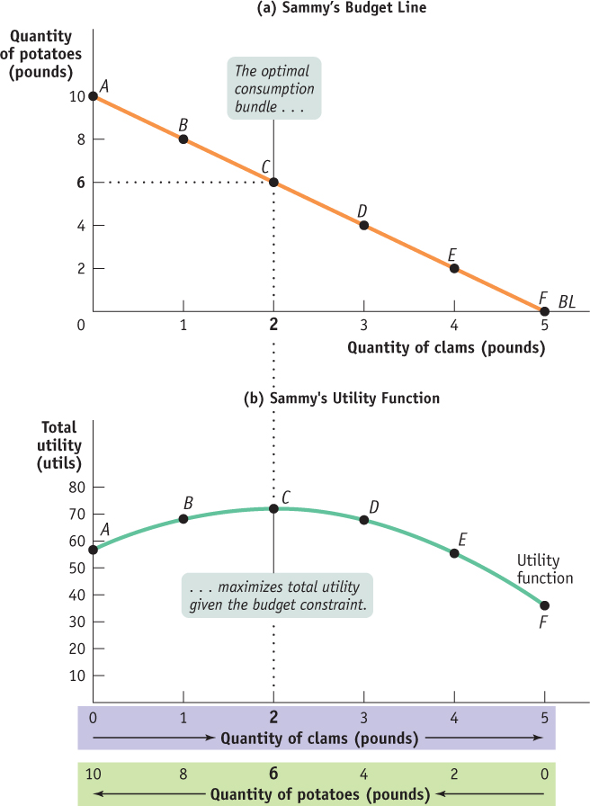
Clearly, the consumption bundle that makes the best of the trade-off between clam consumption and potato consumption, the optimal consumption bundle, is the one that maximizes Sammy’s total utility. That is, Sammy’s optimal consumption bundle puts him at the top of the total utility curve.

As always, we can find the top of the curve by direct observation. We can see from Figure 51.3 that Sammy’s total utility is maximized at point C—that his optimal consumption bundle contains 2 pounds of clams and 6 pounds of potatoes. But we know that we usually gain more insight into “how much” problems when we use marginal analysis. So in the next section we turn to representing and solving the optimal consumption choice problem with marginal analysis.

521