Short-Run Versus Long-Run Costs
AP® Exam Tip
Remember that the long run and the short run don’t refer to predetermined periods of time. They are defined by the degree to which inputs are variable.
Let’s begin by supposing that Selena’s Gourmet Salsas is considering whether to acquire additional food-preparation equipment. Acquiring additional machinery will affect its total cost in two ways. First, the firm will have to either rent or buy the additional equipment; either way, that will mean a higher fixed cost in the short run. Second, if the workers have more equipment, they will be more productive: fewer workers will be needed to produce any given output, so the variable cost for any given output level will be reduced.
The table in Figure 56.1 shows how acquiring an additional machine affects costs. In our original example, we assumed that Selena’s Gourmet Salsas had a fixed cost of $108. The left half of the table shows variable cost as well as total cost and average total cost assuming a fixed cost of $108. The average total cost curve for this level of fixed cost is given by ATC1 in Figure 56.1. Let’s compare that to a situation in which the firm buys additional food-preparation equipment, doubling its fixed cost to $216 but reducing its variable cost at any given level of output. The right half of the table shows the firm’s variable cost, total cost, and average total cost with this higher level of fixed cost. The average total cost curve corresponding to $216 in fixed cost is given by ATC2 in Figure 56.1.
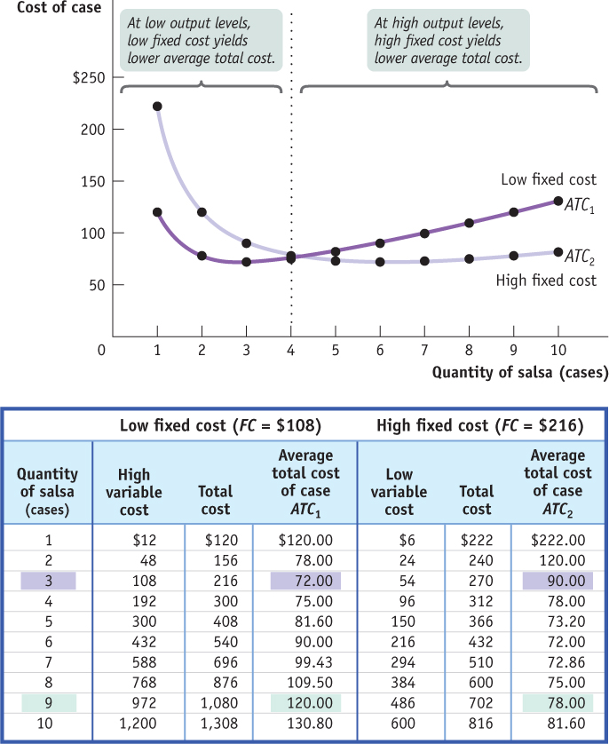
Figure 56.1: Choosing the Level of Fixed Cost for Selena’s Gourmet SalsasThere is a trade-off between higher fixed cost and lower variable cost for any given output level, and vice versa. ATC1 is the average total cost curve corresponding to a fixed cost of $108; it leads to lower fixed cost and higher variable cost. ATC2 is the average total cost curve corresponding to a higher fixed cost of $216 but lower variable cost. At low output levels, at 4 or fewer cases of salsa per day, ATC1 lies below ATC2: average total cost is lower with only $108 in fixed cost. But as output goes up, average total cost is lower with the higher amount of fixed cost, $216: at more than 4 cases of salsa per day, ATC2 lies below ATC1.
From the figure you can see that when output is small, 4 cases of salsa per day or fewer, average total cost is smaller when Selena forgoes the additional equipment and maintains the lower fixed cost of $108: ATC1 lies below ATC2. For example, at 3 cases per day, average total cost is $72 without the additional machinery and $90 with the additional machinery. But as output increases beyond 4 cases per day, the firm’s average total cost is lower if it acquires the additional equipment, raising its fixed cost to $216. For example, at 9 cases of salsa per day, average total cost is $120 when fixed cost is $108 but only $78 when fixed cost is $216.
Why does average total cost change like this when fixed cost increases? When output is low, the increase in fixed cost from the additional equipment outweighs the reduction in variable cost from higher worker productivity—that is, there are too few units of output over which to spread the additional fixed cost. So if Selena plans to produce 4 or fewer cases per day, she would be better off choosing the lower level of fixed cost, $108, to achieve a lower average total cost of production. When planned output is high, however, she should acquire the additional machinery.
In general, for each output level there is some choice of fixed cost that minimizes the firm’s average total cost for that output level. So when the firm has a desired output level that it expects to maintain over time, it should choose the optimal fixed cost for that level—that is, the level of fixed cost that minimizes its average total cost.
Now that we are studying a situation in which fixed cost can change, we need to take time into account when discussing average total cost. All of the average total cost curves we have considered until now are defined for a given level of fixed cost—that is, they are defined for the short run, the period of time over which fixed cost doesn’t vary. To reinforce that distinction, for the rest of this module we will refer to these average total cost curves as “short-run average total cost curves.”
For most firms, it is realistic to assume that there are many possible choices of fixed cost, not just two. The implication: for such a firm, many possible short-run average total cost curves will exist, each corresponding to a different choice of fixed cost and so giving rise to what is called a firm’s “family” of short-run average total cost curves.
At any given time, a firm will find itself on one of its short-run cost curves, the one corresponding to its current level of fixed cost; a change in output will cause it to move along that curve. If the firm expects that change in output level to be long-standing, then it is likely that the firm’s current level of fixed cost is no longer optimal. Given sufficient time, it will want to adjust its fixed cost to a new level that minimizes average total cost for its new output level. For example, if Selena had been producing 2 cases of salsa per day with a fixed cost of $108 but found herself increasing her output to 8 cases per day for the foreseeable future, then in the long run she should purchase more equipment and increase her fixed cost to a level that minimizes average total cost at the 8-cases-per-day output level.
The long-run average total cost curve shows the relationship between output and average total cost when fixed cost has been chosen to minimize average total cost for each level of output.
Suppose we do a thought experiment and calculate the lowest possible average total cost that can be achieved for each output level if the firm were to choose its fixed cost for each output level. Economists have given this thought experiment a name: the long-run average total cost curve. Specifically, the long-run average total cost curve, or LRATC, is the relationship between output and average total cost when fixed cost has been chosen to minimize average total cost for each level of output. If there are many possible choices of fixed cost, the long-run average total cost curve will have the familiar, smooth U shape, as shown by LRATC in Figure 56.2.
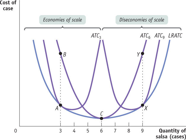
Figure 56.2: Short-Run and Long-Run Average Total Cost CurvesShort-run and long-run average total cost curves differ because a firm can choose its fixed cost in the long run. If Selena has chosen the level of fixed cost that minimizes short-run average total cost at an output of 6 cases, and actually produces 6 cases, then she will be at point C on LRATC and ATC6. But if she produces only 3 cases, she will move to point B. If she expects to produce only 3 cases for a long time, in the long run she will reduce her fixed cost and move to point A on ATC3. Likewise, if she produces 9 cases (putting her at point Y) and expects to continue this for a long time, she will increase her fixed cost in the long run and move to point X.
We can now draw the distinction between the short run and the long run more fully. In the long run, when a producer has had time to choose the fixed cost appropriate for its desired level of output, that producer will be at some point on the long-run average total cost curve. But if the output level is altered, the firm will no longer be on its long-run average total cost curve and will instead be moving along its current short-run average total cost curve. It will not be on its long-run average total cost curve again until it readjusts its fixed cost for its new output level.
Figure 56.2 illustrates this point. The curve ATC3 shows short-run average total cost if Selena has chosen the level of fixed cost that minimizes average total cost at an output of 3 cases of salsa per day. This is confirmed by the fact that at 3 cases per day, ATC3 touches LRATC, the long-run average total cost curve. Similarly, ATC6 shows short-run average total cost if Selena has chosen the level of fixed cost that minimizes average total cost if her output is 6 cases per day. It touches LRATC at 6 cases per day. And ATC9 shows short-run average total cost if Selena has chosen the level of fixed cost that minimizes average total cost if her output is 9 cases per day. It touches LRATC at 9 cases per day.

Photodisc
Suppose that Selena initially chose to be on ATC6. If she actually produces 6 cases of salsa per day, her firm will be at point C on both its short-run and long-run average total cost curves. Suppose, however, that Selena ends up producing only 3 cases of salsa per day. In the short run, her average total cost is indicated by point B on ATC6; it is no longer on LRATC. If Selena had known that she would be producing only 3 cases per day, she would have been better off choosing a lower level of fixed cost, the one corresponding to ATC3, thereby achieving a lower average total cost. Then her firm would have found itself at point A on the long-run average total cost curve, which lies below point B.
AP® Exam Tip
Don’t mix up the concepts of diminishing returns and returns to scale. Diminishing returns is a short-run concept because at least one input is being held constant. Returns to scale is a long-run concept because all inputs are variable.
Suppose, conversely, that Selena ends up producing 9 cases per day even though she initially chose to be on ATC6. In the short run her average total cost is indicated by point Y on ATC6. But she would be better off purchasing more equipment and incurring a higher fixed cost in order to reduce her variable cost and move to ATC9. This would allow her to reach point X on the long-run average total cost curve, which lies below Y. The distinction between short-run and long-run average total costs is extremely important in making sense of how real firms operate over time. A company that has to increase output suddenly to meet a surge in demand will typically find that in the short run its average total cost rises sharply because it is hard to get extra production out of existing facilities. But given time to build new factories or add machinery, short-run average total cost falls.
Returns to Scale
There are economies of scale when long-run average total cost declines as output increases.
There are increasing returns to scale when output increases more than in proportion to an increase in all inputs. For example, with increasing returns to scale, doubling all inputs would cause output to more than double.
What determines the shape of the long-run average total cost curve? It is the influence of scale, the size of a firm’s operations, on its long-run average total cost of production. Firms that experience scale effects in production find that their long-run average total cost changes substantially depending on the quantity of output they produce. There are economies of scale when long-run average total cost declines as output increases. As you can see in Figure 56.2, Selena’s Gourmet Salsas experiences economies of scale over output levels ranging from 0 up to 6 cases of salsa per day—the output levels over which the long-run average total cost curve is declining. Economies of scale can result from increasing returns to scale, which exist when output increases more than in proportion to an increase in all inputs. For example, if Selena could double all of her inputs and make more than twice as much salsa, she would be experiencing increasing returns to scale. With twice the inputs (and costs) and more than twice the salsa, she would be enjoying decreasing long-run average total costs, and thus economies of scale. Increasing returns to scale therefore imply economies of scale, although economies of scale exist whenever long-run average total cost is falling, whether or not all inputs are increasing by the same proportion.
There are diseconomies of scale when long-run average total cost increases as output increases.
There are decreasing returns to scale when output increases less than in proportion to an increase in all inputs.
There are constant returns to scale when output increases directly in proportion to an increase in all inputs.
In contrast, there are diseconomies of scale when long-run average total cost increases as output increases. For Selena’s Gourmet Salsas, decreasing returns to scale occur at output levels greater than 6 cases, the output levels over which its long-run average total cost curve is rising. Diseconomies of scale can result from decreasing returns to scale, which exist when output increases less than in proportion to an increase in all inputs—doubling the inputs results in less than double the output. When output increases directly in proportion to an increase in all inputs—doubling the inputs results in double the output—the firm is experiencing constant returns to scale.
What explains these scale effects in production? The answer ultimately lies in the firm’s technology of production. Economies of scale often arise from the increased specialization that larger output levels allow—a larger scale of operation means that individual workers can limit themselves to more specialized tasks, becoming more skilled and efficient at doing them. Another source of economies of scale is a very large initial setup cost; in some industries—such as auto manufacturing, electricity generating, and petroleum refining—it is necessary to pay a high fixed cost in the form of plant and equipment before producing any output. A third source of economies of scale, found in certain high-tech industries such as software development, is network externalities, a topic covered in a later module. As we’ll see when we study monopoly, increasing returns have very important implications for how firms and industries behave and interact.
AP® Exam Tip
Firms with increasing returns to scale benefit from their larger size as long-run average total cost decreases with increased output, while firms with decreasing returns to scale are hurt by their size as long-run average total cost rises with increased output.
Diseconomies of scale—the opposite scenario—typically arise in large firms due to problems of coordination and communication: as a firm grows in size, it becomes ever more difficult and therefore costly to communicate and to organize activities. Although economies of scale induce firms to grow larger, diseconomies of scale tend to limit their size.